Download a .pdf copy here…Part 1 Part
2
Introduction
to Using the TI-89 Calculator
|
Note: If this is the first
time that you have used the TI-89 computer algebra system (CAS) calculator
then you should first work through this Introduction to Using the TI-89,
otherwise jump to the section Using the TI-89 in Mathematics. Some of the
information found there in terms of key presses, menus, etc. will be assumed
in what follows. While much of the information provided here describes how to
carry out many mathematical procedures on the TI-89, using technology is not
simply about finding answers, and we would encourage you NOT to see this
calculator as primarily a quick way to get answers. Research by the authors,
and others, shows that those who do this tend to come to rely on the
calculator to the detriment of their mathematical understanding. Instead
learn to see the TI-89 as a problem-solving, and investigative tool that will
help you to understand concepts by providing different ways of looking at
problems, thus helping you reflect on the underlying mathematics.
|
1.
Saying
'Hello' to your graphics calculator
|
Instructions
|
TI-89
|
|
You will use the following keys.
a) Press
The calculator cursor should be in the
Home Screen (see the black cursor flashing in the bottom left hand corner).
·
Press
2
The calculator should
turn off.
·
If
you can’t see the screen use • ´
(darker) or • | (lighter) to change screen contrast.
· [HOME] displays the Home Screen,
where you perform most calculations.
|

|
Basic
Facilities of the TI-89
|
Function Keys
|
Cursor Pad
|
|
[F1]
through [F8] function keys let you select toolbar menus.

|
The cursor is controlled by the large blue circle on the top
right hand side of the calculator. This allows access to any part of an
expression.

|
|
Application Short Keys
|
Calculator
Keypad
|
|
Used
with the • key to let you select
commonly used applications:
[Y=]
[WINDOW] [GRAPH] [TblSet] [TABLE]
|
 Performs a variety of
mathematical and scientific operations. Performs a variety of
mathematical and scientific operations.
|
2 • § and j modify the action of other keys:
|
Modifier
|
Description
|
|
2
(Second)
|
Accesses
the second function of the next key you press
|
|
•
(Diamond)
|
Activates “shortcut” keys that selects
applications and certain menu items directly from the keyboard.
|
|
§
(Shift)
|
Types an uppercase character for the next letter key
you press.
|
|
j
|
Used to type alphabetic letters,
including a space character. On the keyboard, these are printed in the same
colour as the j key.
2 j used to
type alphabetic letters.
|
|
|
Key
|
Description
|
|
O
|
Displays a
menu that lists all the applications available on the TI-89.
|
|
N
|
Cancels any
menu or dialogue box.
|
|
∏
|
Evaluates an expression, executes an instruction,
selects a menu item, etc.
|
|
3
|
Displays a list of the TI-89’s current mode settings,
which determine how numbers and graphs are interpreted, calculated, and
displayed.
|
|
M
|
Clears
(erases) the entry line.
|
|
|
[CATALOG]
|
Press b or c to
move the d indicator to the function or instruction. (You can move quickly
down the list by typing the first letter of the item you need.)
Press ∏. Your
selection is pasted on the home screen.
|
|
Application
|
Lets you:
|
|
[Home]
|
Enter expressions and instructions, and
performs calculations
|
|
[Y= ]
|
Define, edit, and select functions or
equations for graphing
|
|
[Window]
|
Set window dimensions for viewing a graph
|
|
[Graph]
|
Display graph
|
|
[Table]
|
Display a table of variable values that
correspond to an entered function
|
|
Press:
|
To
display
|
|
F1, F2,
etc.
|
A toolbar
menu– Drops down from the toolbar at the top of most application screens.
Lets you select operations useful for that application
|
|
[CHAR]
|
CHAR menu– Lets you select from categories of special characters
(Greek, math, etc.)
|
|
[MATH]
|
MATH menu– Lets you select from
categories of mathematical operations
|
|
Press
|
To perform
|
|
2 [F6]
|
Clean
Up to start a new problem:
|
|
Clear
a–z
|
Clears (deletes) all single-character
variable names in the current folder.
If any of the
variables have already been assigned a value, your calculation may produce
misleading results.
|
|
Problem?
|
Try this!
|
|
If you make a typing error
|
If you make
a typing error use 0 to undo one character
at a time
If
necessary, also press M to clear the complete line.
|
|
If you want to clear the home screen completely
|
Press F1 n
|
Mode
Settings
|
Instructions
|
Screen Shot
|
|
Press 3, which
shows the modes and their current settings
|
|
|
If you
press F2 then ‘Split Screen’ specifies how the
parts are arranged: FULL (no split screen), TOP-BOTTOM, or LEFT-RIGHT
|
|
(a)
Entering
a Negative Number
|
Instructions
|
Examples
|
|
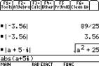
Use | for subtraction and use ∑ for negation.
To
enter a negative number, press ∑
followed by the number.
|
To enter the number –7, press ∑ 7.
9 p ∑ 7 = –63,
9 p | 7 = displays an
error message
To calculate –3 – 4, press ∑ 3 | 4
|
(b)
Implied Multiplication
|
If you enter:
|
The TI-89 interprets it as:
|
|
2a
|
2*a
|
|
xy
|
Single variable named xy; TI-89 does not read as x*y
|
(c)
Substitution
|
Instructions
|
Examples
|
|
Using 2 [ | ]key
|
eg) ∑ x^2+2 x x=3 –7
This
calculates the value of –x2 + 2
when x = 3
|
|
 Using ‘STORE’ key: ß Using ‘STORE’ key: ß
|
eg) Find f(2) if 
∑ x^3+2 ß f(x) –x3 + 2® f(x)
f(2) -6 –6
|
(d)
Rational Function Entry
|
Instructions
|
Example
|
|
 = (numerator) e (denominator ) = (numerator) e (denominator )
|
 ® (x + 1) e (2x – 1) ® (x + 1) e (2x – 1)
|
(e)
Operators
|
addition: +
|
subtraction : –
|
multiplication: ´
|
division: 
|
Exponent: ^
|
(f)
Elementary Functions
|
Exponential: e^(x)
|
Trigonometric:
|
|
natural
logarithm: ln(x)
square
root: Ö
absolute
value: abs(x)
|
sin(x), cos(x), tan(x), sin-1(x), cos-1(x), tan-1(x)
If you want sec(x) then put 1/cos(x) , cosec(x) is 1/sin(x).
Note: The
trigonometric functions in TI-89 angles are available in both degrees and
radians. If you want degrees (180°) or radians (p)
change using the 3 key previously discussed.
|
(g)
Constants
|
To find:
|
Work
|
|
i : imaginary
number
|
with 2 key
|
|
p : Pi
|
with 2 key
|
|
¥ : infinity
|
with • key
|
(h)
 Recalling the last answer
|
Instructions
|
Example
|
|
2 ±
|
ans(1) Contains
the last answer
ans(2) Contains
the next-to-last answer
|
(i)
Cutting, Copying and Pasting
|
Press:
|
To:
|
|
§ B or
§ A
|
highlight the expression.
|
|
•
5, • 6 and • 7
|
cut, copy and paste.
|
|
2 ≤
|
replace the contents of the entry line with any previous
entry.
|
(j) When differentiating with respect to x
|
To find:
|
Type:
|
|
Limit  : :
|
lim( f(x), x , a )
|
|
Indefinite
Integral  : :
|
 ( f(x) , x, c ) ( f(x) , x, c )
|
|
Definite
integral  : :
|
 ( f(x), x, a, b) ( f(x), x, a, b)
|
|
Area
between f(x) and g(x) on the interval [a, b]:
|

|
|
Differentiation
 : :
|
d( f(x) , x )
|
(b) Table
|
Instructions
|
Screen Shot
|
|
Press • [TABLE] to
see the table of values for 2x + 3, as shown
below:
|
|
|
Press • [TblSet],
try change the settings and see the effect in [TABLE].
|
|
|
|

|
|
|
|
|
|
|
|
Instructions
|
Screen Shot
|
|
By changing [TblSet] from [1. AUTO] to [2.ASK], complete
the table below:
Remember: y1 is still set to 2x + 3
|

|
|
|
|
3. Graphing
(a) Displaying Window Variable in the Window Editor
|
Instructions
|
Screen
Shot
|
|
Press • [WINDOW] or O 3 to display the Window Editor.
|
|
|
|
|
|
Variables
|
Description
|
|
xmin, xmax, ymin, ymax
|
Boundaries of the viewing window.
|
|
xscl, yscl
|
These x
and y scales set the distance between tick
marks on the x and y axes (see above right)..
|
|
xres
|
Sets pixel resolution (1 through 10) for
function graphs. The default is 2.
|
(b) Overview of the Math Menu
|
|
|
|
Press F5 from the Graph screen
|
|
|
Math
Tool
|
Description
|
|
Value
|
Evaluates
a selected y(x)
function at a specified x value
|
|
Zero,
Minimum, Maximum
|
Finds a
zero (x-intercept), minimum, or maximum point
within an interval.
|
|
Intersection
|
Finds the intersection of two functions.
|
|
Derivatives
|
Finds the derivative (slope) at a point.
|
|

|
Finds the approximate numerical integral
over an interval.
|
|
A:Tangent
|
Draws a tangent line at a point and
displays its equation
|
(b) Finding the Maximum & Minimum Values of a Function from its
Graph
|
Instructions
|
Screen
Shot
|
|
1. Display
the Y=Editor.
|
|
|
2. Enter the function
|
|
|
3. Enter
graph mode (• F3). Open the Math Menu F5, and
select 4: Maximum.
|
|
|
4. Set the
lower bound.
|
|
|
5. Set the
upper bound.
|
|
|
6. Find the maximum point on
the graph between the lower and upper bounds.
|
|
|
7. Transfer
the result to the Home screen, and then display the Home screen.
[Home]
|
|
(c) Overview of the Zoom Menu
|
Instructions
|
Screen Shot
|
|
Press F2 from y=Editor, window Editor, or Graph screen
|
|
|
Zoom
tool
|
Description
|
|
1:ZoomBox
|
Lets you
draw a box and zoom in on that box.
|
|
2:ZoomIn 3:ZoomOut
|
Lets you select a point and zoom in or
out by an amount defined by SetFactors.
|
|
4:ZoomDec
|
Sets Dx and Dy to 0.1, and centres the origin.
|
|
6:ZoomStd
|
Sets Window variables to their default
values.
xmin= –10,
xmax= 10, xscl=1,
ymin= –10, ymax=
10, yscl= 1, xres=
2
|
|
Note: To get out of the graphing mode use 2 K.
This will not work
while the BUSY icon is
flashing in the bottom right hand corner.
Adjust your graph by
selecting F2 and choosing 2:ZoomIn,
3:ZoomOut, or A:ZoomFit
|
Example: Graph  by following these instructions.
|
Instructions
|
Screen Shot
|
|
• # x ^ 2 ∏
|
|
|
• %
|
|
To draw a new graph go to [y=] and change the formula in the y1 position using the cursor to move up to it to delete it. This effectively clears the previous graph as well.
Alternatively, using y2 will add the new graph to y = x2.
[HOME] returns you to the Home screen.
4. The Algebra Menu
|
Menu Item
|
Description F2 MENU
|
|
|
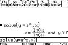
1: solve
|
Solves an expression for a specified
variable. This returns solutions only, regardless of the Complex Format mode
setting (For complex solutions, select A:Complex from the algebra menu).
|
|
2: factor
|
Factorises an expression with respect to
all its variables or with respect to only a specified variable.
|
|
3: expand
|
Expands an expression with respect to all
its variables or with respect to only a specified variable.
|
|
4: zeros
|
Determines the values of a specified
variable that make an expression equal to zero.
|
|
5: approx
|
Evaluates an expression using
floating-point arithmetic, where possible.
|
|
6: comDenom
|
Calculates a common denominator for all
terms in an expression and transforms the expression into a reduced ratio of
a numerator and denominator.
|
|
7: propFrac
|
Returns an expression as a proper
fraction expression.
|
Using the TI-89 in Mathematics
Topic 0
Preliminaries
0.2
Inequalities and the absolute value
|
Instructions
|
Screen Shot
|
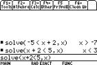
Inequalities
We can directly solve these, for example
3x – 2 ≥ 7x +10
F2
3x | 2 • √ 7x ´ 10 b x d ∏
|
|
|
We can also transform an inequality into
the form x ≥ or x ≤ by performing the same operation on both sides.
For example we can solve the inequality
3x – 2 ≥ 7x +10 ∏
by adding –7x to both sides of the equation, then adding 2
2 ± | 7x ∏
2 ± ´ 2 ∏
|
|
|
and dividing by –4 gives the answer.
2
± e ∑ 4 ∏
Note that the CAS reverses the inequality
when dividing by the –ve quantity.
|
|
|
The absolute value function is found in
the I menu (press 2
5), select 1: Number, select 2: abs( (or Press D and ∏) and press ∏.
(This function also gives the modulus of
a complex number.). To switch from exact to approximate
mode we press • ∏.
|
|
|
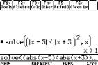
Inequalities with absolute values can be
solved when they are broken down into single inequalities,
|
|
|
or sometimes by squaring both sides of
the inequality (note the unusual notation for this).
F2 1: Solve( ( 2 5 1: Number 2: abs( x–5)< (2 5 1: Number 2: abs( x+3))^2, x)
|
|
|
Note: The use of the • key to
switch between exact and approximate modes (the TI-89 tries to use fractions
in exact mode).
|
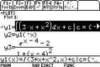
0.3 Domain, range and graph of a function
|
Instructions
|
Screen Shot
|
|
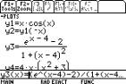
We can use the
[Y= ] menu obtained by pressing • [Y= ] to draw graphs. Place the
cursor just to the right of y1= and enter the
function required. Note that we can use previously defined functions in later
ones.
|
|
|
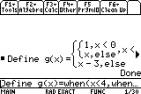
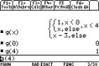
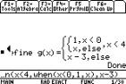
To enter a split domain function we use
the when ( ) function and nest them if there are more than two parts to the
piecewise function. This has been done by defining a function g and using y1= g.
|
|
|
We can use g a number of times this way.
|

|
|
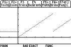
Note that
these graphs look better when
plotted in
the dot style. This found on the
[Y= ] screen under F6 Style, 2:
Dot.
|

|
|
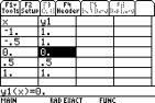
We can test the value of the function g
at the points x=0, and x=4 on the [HOME] screen, as shown.
|
|
|
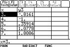
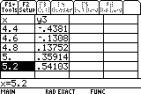
Or we could use a table of values.
|
|
|
Note: Use • &to
zoom in on the table values.
|
0.4 Trigonometric functions
|
Instructions
|
Screen Shot
|
|
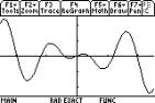
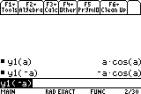
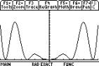
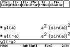
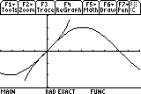
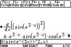
The graphs
of the functions f(x)=xcos(x) and f(x)=x2sin2(x) (entered as sin(x)^2) are
shown on the TI-89. We can verify that one is an odd
function and the other even, by checking f(a)
against f(–a) on the [HOME] screen.
|
|
|
It’s an odd function.
|
|
|
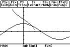
Graph of the
function
f(x)=x2sin2(x)
|
|
|
It’s an even function.
|
|
0.5 Translations and compositions
of functions
|
Instructions
|
Screen Shot
|
|
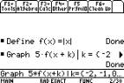
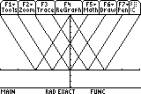
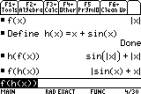
We can check the effect of a
transformation by looking at multiple graphs of a function, using the |
command to set values of a variable (which can be read as ‘when’).
Enter F4 1: Define j F(x)= 2 5 1: Number 2:
abs(x)
|
|
|
|

|
|
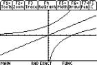
The graph
function is at F4 Other 2: Graph
|
|
|
Composite functions can be obtained from previously defined functions using the
notation f(g(x)).
|
|
0.6 0ne-to-one and inverse
functions
|
Instructions
|
Screen Shot
|
|
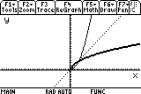
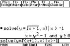
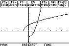
Graphs of functions which are inverses,
such as exp and ln will not look like reflections in y=x on the TI-89 unless the same scale can be used on each axis.
|
|
|
This can be done using F2 Zoom 5: Zoom
Sqr (as shown in these graphs).
|
|
|
Note there is also a function in graph mode
F6 Draw 3; DrawInv to draw an inverse function’s graph
|
|
|
The inverse trig functions are provided on the TI-89 and their domains are known by the
calculator.
sin–1 is at • Y.
|
|
|
|
|
|
|

|
|
|
|
|
|
|
|
Note: We can not use f(x)^–1 for inverse functions. This gives the reciprocal of the
function.
|
Topic 1 Limits
1.1 Limits of a function
|
Instructions
|
Screen Shot
|
|
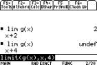
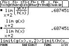
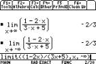
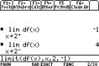
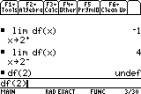
Use F3 3:
Limit( to find limits. The order
is Limit(function, variable, value
approached).
|
|
|
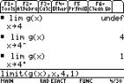
We can also
find one-sided limits by
writing 1 or –1 before closing the bracket
for right
and left limits respectively (NB
do NOT enter +1, only 1). If the limit does not exist we are given the
answer undef(ined). Checking the right and left limits may help us see why
this is so.
|
|
|
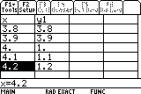
Checking a
table of values can also be
useful.
|
|
|
While not proving them, we can verify
limit laws for some examples. You should check them with some functions of
your own. Note the use of the calculator’s approximate mode here.
|
|
Example 1.1
|
Instructions
|
Screen
Shot
|
|
Example 
Some limits
do not exist. We can build an understanding of some reasons for this.
|
|
|
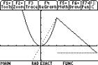
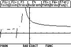
We can plot
the graph and zoom in on
x = 0.
|
|
|
Or from the table we can see that no
matter how much we zoom in on x = 0 values do
not tend towards the same number (left and right limits do not exist).
|
|
|
|
|
|
|
|
Example 1.2
|
Instructions
|
Screen
Shot
|
|
Example:
Find 
This is an
important limit, but one that cannot be found by putting x = 0, since the function is undefined for x = 0. Enter
F3 ™ f(x) = W x d e x b x b µ d ∏
|
|
|
If we change
the value of x, taking steps closer to 0 then
the value of f(x) gets closer to 1.
|
F3 ™ f(x) = W x d e x b x b µ d ∏
|
F3 ™ f(x) b x b µ d ∏
|
|
|
|
Looking at the graph can help with what the limit might
be.
|
|
|
We can use a table…
|
|
|
|
|
|
|

|
|
We find that:
 = 1 = 1
|
|
1.3 Continuity
|
Instructions
|
Screen
Shot
|
|
The function g used in 0.3 is discontinuous at x=0
and x=4. The limits at x=4 were calculated in Example 1.1.
|
|
|
|
|
|
To be continuous at x=4 we would need the right limit to equal the left.
|

|
1.3.2
The
intermediate value theorem
|
Instructions
|
Screen Shot
|
|
This is very
useful for showing that there
is a root of
f(x)=0 between two domain
values. If f(a)<0 and f(b)>0 (or vice versa) then there
is a zero of f between a and b. Using the table of values in a graph we can then zoom in on the
root.
|

|
|
For the
function below we see from the
table that f(4)<0 and f(5)>0, so we zoom
in to find
the root, using the Intermediate
Value
Theorem.
|
|
|
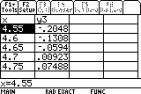
This table
shows it is between 4.6 and 4.8. and
|
|
|
This table
shows it is between 4.65 and
4.7. This
can be continued to the required accuracy.
|
|
|
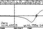
We could of
course get the TI-89 to find the root directly from the [Graph] or [Home]
screens, but we need to understand that this theorem is one basis for finding
it. For the graph use F5 Math, 2: Zero, enter the lower and upper bounds (4
and 5 from the theorem) and we get 4.69315 for the root of f(x)=0 or the zero of f.
|
|
|
In the [Home] screen we use F2 1: Solve
( and enter f(x)=0, x). We need
approximate mode (holding down • when
pressing ∏) to get the decimal answer.
|

|
1.4
Limits involving infinity
|
Instructions
|
Screen Shot
|
|
Limits involving infinity are entered as
before but using * key (• Ω)as if it is the value approached.
|
|
1.4.3 Asymptotes
|
Instructions
|
Screen Shot
|
|
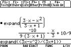
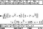
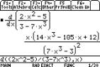
Use the limits to find the horizontal
asymptotes. For sloping asymptotes we can use the TI-89 to divide the
numerator of a function by its denominator, using F2, 3: Expand (the function
F2, 7: propFrac( will give the same result here). The asymptote here is y=–x/3 + 10/9 since as x®¥ the remainder of the expansion approaches 0.
|
|
|
The answer can be checked by drawing both
graphs.
|
|
2.1 Tangents and rate of change
|
Instructions
|
Screen Shot
|
|
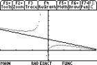
Consider the function y=x2. We can define a rate of change function r to be the gradient of a chord of length h. That is:  (NB there is a
built-in numeric derivative function at F3 A: nDeriv which could be used but
looks rather different).
We can then use this function r at a point, for example, x = 2. Whenever we
change h taking steps of h closer to 0 then the value of r is
getting closer to 4. (NB there is a
built-in numeric derivative function at F3 A: nDeriv which could be used but
looks rather different).
We can then use this function r at a point, for example, x = 2. Whenever we
change h taking steps of h closer to 0 then the value of r is
getting closer to 4.
|
|
|
We can
confirm this by asking for the limit of r as h approaches 0.
|
|
|
Note: 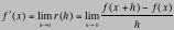 (where the
limits exist). Thus here the rate of change at x = 2: (where the
limits exist). Thus here the rate of change at x = 2: 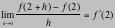 = 4. = 4.
|
2.2
The derivative as a function
|
Instructions
|
Screen Shot
|
|
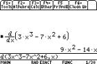
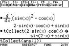
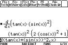
To
differentiate on the TI-89 we use the F3 Calc, 1: d( differentiate command, which is also found at 2 n. The
format is d(function, variable to
differentiate with respect to).
|
|
|
In the
second example we can use the
function
Trig collect, found in F2, 9:
Trig, 2:
tCollect to simplify the answer.
Use 2 ∑ for ANS,
the previous answer.
|
|
Example 2.1
|
Instructions
|
Screen Shot
|
|
Find out whether the function is differentiable at x=2. is differentiable at x=2.
Define the piecewise functions by using
the following instructions.
F4 ® f(x) = when c x 2 ¬ 2 b x Z 2 b 6 | x d ∏
Then we graph the function f . We can define a function Df as
its derivative  (use F6 2: Dot
in [Y=] to plot the derivative). Note that this may not be defined on the
whole domain. (use F6 2: Dot
in [Y=] to plot the derivative). Note that this may not be defined on the
whole domain.
We can see the discontinuity in the
derived function’s graph, but must check the limits on the "
screen.
|
|
|
Right limit is: F3 ™ df(x) b x b 2 b 1 d ∏
Left limit is: F3 ™ df(x) b x b 2 b ∑1 d ∏
|
|
|
Since the limits are not the same the function
is not differentiable at x=2 and df(2) is undefined.
|
|
Example 2.2
|
Instructions
|
Screen Shot
|
|
Example. Find the derivative of f(x) = xn
Define the function f(x) = xn. When we define the value of power, n = 1, 2, 3, 4, 10 the functions are changed to the
actual functions, x, x2, x3, x4, x10.
|
|
|
If we define the slope function r as the average rate of change,
|
|
|
|
|
|
then we can see that the derivative of the functions are
1, 2x, 3x2, 4x3, 10x9.
|
|
|
Using the rate of function r, we can
get that the general derivative of xn is
nxn-1
|
|
|
Thus 
|
|
2.2.1 Second and higher derivatives
|
Instructions
|
Screen Shot
|
|
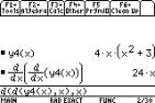
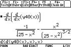
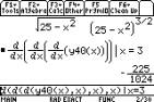
These can be accomplished by using
repeated applications of the CAS function d.
Here functions y4(x) and y40(x) from the [Y= ] list have been used. Note the inclusion of the
variable each time and the option of finding the value of a derivative at a
specific value of x.
|
|
|
|
|
|
|
|
|
Alternatively we can specify the nth derivative with F3 1: d(
differentiate function, x, n)
|
|
2.3 Differentiation rules
|
Instructions
|
Screen Shot
|
|
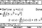
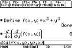
The TI-89 can act on functions that are
unknown, to give the differentiation formulas.
|
|
|
|
|
|
The common denominator function F2 6:
comDenom( has been used to simplify an answer by combining two terms over a
common denominator.
|
|
|
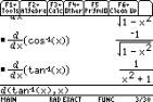
Otherwise the TI-89 can be used to check differentiation
of these functions by direct entry, as here.
|
|
|
|
|
|
|
|
2.4 The Chain Rule
|
Instructions
|
Screen Shot
|
|
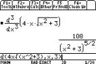
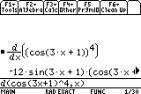
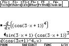
The rule for this can be seen similarly for f(x)
raised to the power of n.
|
|
|
Again functions are entered directly, although we can
define them separately.
|

|
|
|
|
|
|
|
|
|
|
2.5 Implicit differentiation
|
Instructions
|
Screen
Shots
|
|
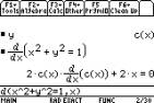
This can be accomplished by defining y to be some function of x, here c.
|
|
|
|
|
|
Inverse trig functions are entered
directly.
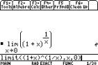
|
|
|
The TI-89 confirms the value of the limit
giving e.
|
|
|
Note the asymptote at x=–1.
|
|
3.1 Maximum and minimum values and
3.2 Derivatives and the shapes of curves
|
Instructions
|
Screen Shots
|
|
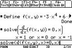
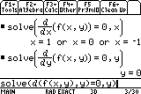
Relative Extrema: Find all relative
extrema of the function g(x)=x3–9x2+24x–7 and confirm your result by sketching the graph. The TI-89
method combines use of the differentiation command, the solve command for  ,… ,…
|
|
|
graphs of the function and its derivative
to relate the algebraic solution to the pictures,…
|
|
|
|
|
|
and a table of values to get coordinates
of points, check limits, etc.
|

|
|
|
|
Example 3.1
|
Instructions
|
Screen Shot
|
|
Find the relative maximum and minimum values of the
function
f(x) = x3 – x.
First we can get an idea of the solutions
by sketching the graphs of the function and its derivative.
|
|
|
Note the use of y2(x)= to sketch the graph of the derivative. to sketch the graph of the derivative.
|
|
|
|
|
|
|
|
|
Answers obtained from using F5 Maths 3:
Minimum or 4: Maximum from the graph screen can be checked algebraically for
accuracy in the [HOME] screen.
|
|
|
|
|
Example 3.2
|
|
|
|
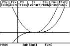
The derivative can be zero without there
being a relative maximum or relative minimum.
Example. f(x) = x3 – 3x2 + 3x – 1
|
|
|
|
|
|
|
|
|
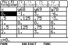
The second derivative test can be used to
confirm that we have a point of inflection at x=1. Put y3(x) equal to the second derivative and view the table of values,
around x=1. We see that  changes sign
from negative to positive through x=1 (and is
zero at x=1, check on the [HOME] screen and
note the Intermediate Value Theorem) and so we have a point of inflection (y68=f, y69= changes sign
from negative to positive through x=1 (and is
zero at x=1, check on the [HOME] screen and
note the Intermediate Value Theorem) and so we have a point of inflection (y68=f, y69= and y70= and y70= here). here).
|
|
|
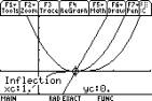
We can check this on the graph screen by
using F5 Maths 8: Inflection.
|
|
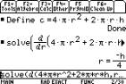
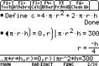
3.3 Optimisation problems
|
Instructions
|
Screen Shot
|
|
Often in these questions we have to find
the optimum value of a function of two or more variables by first
substituting for one of the variables a function previously formed. This can
be done in a relatively easy way on the TI-89. Taking example 2 on the manual
in section 3.3, we have to minimise the cost,  subject to subject to  . Note that the form of the condition (using | ) means that
the answer comes out well or does not come out at all. . Note that the form of the condition (using | ) means that
the answer comes out well or does not come out at all.
|
|
|
|
|
|
|
|
|
|

|
3.4 Antidifferentiation
|
Instructions
|
Screen Shot
|
|
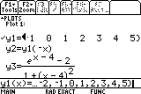
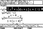
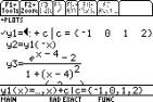
Use the symbol ∫ found at 2 m for the
antiderivative. We can enter on the [Y= ] screen the function y1(x) = 2 m function, x) + c when c={list of values separated by commas}. This will give us a number
of antiderivatives of the function.
|
|
|
y1 is then
the function F(x).
|
|
|
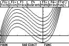
Graphing the function will show what
these functions look like and the relationship between them.
|
|
|
|
|
|
|
|
|
Since they only differ by a constant the
graphs are all translations of each other parallel to the y-axis.
|
|
Displacement,
velocity and acceleration
|
Instructions
|
Screen Shot
|
|
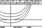
Set the graph drawing mode to
differential equations using MODE Graph 6: DIFF EQUATIONS. In the Y= mode the
DEs are then set up ready for you to enter. The TI-89 uses t not x.
The variable t is given a key of its own on the TI-89, like x, y, and z namely ‹.
|
|
|
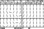
To draw a direction field using the
TI-89.
|
|
|
|
|
|
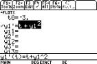
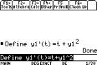
Select the [Y= ] screen and enter the
differential equation using t (and Y1—or Yn—if needed). There is no use
of x.
Use • [Window] (F2) to set
the window dimensions to an appropriate t and Y size. Choose ‘GRAPH’ and it will put in the direction field.
|
|
|
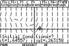
Selecting F8 IC enables a particular
antiderivative solution to be drawn: IC stands for Initial Conditions,
meaning a point (or points) known to be on the graph of the antiderivative
required. Enter the co-ordinates or move the cursor to a chosen point and
press ENTER.
|
|
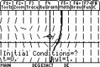
|
The solution curves for the
antiderivative through the given point(s) is drawn.
|

|
|
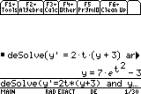
To solve a DE algebraically we use the
command F3 C: deSolve(
Use 2 = for the  . .
Example 189 use
F3 C: deSolve( y2 = = 2t(y+3) and y(0)=4, t, y)
|
|
|
|

|
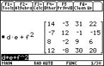
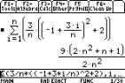
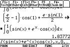
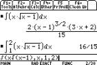
4. Integration
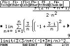
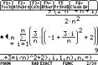
4.1 The area problem
To find the area under the curve f(x) =
x2 + 2, from x = –1 to x = 2. using rightsum we
have
x0 = –1, x1 = –1 + 3/n, x2 = –1 + 2.3/n,… xi = –1 + 3i/n,… xn = –1 + 3n/n
= –1+3=2.
So the area can be obtained by taking the
limit (if it exists) of the Riemann sum as n ®∞.
Area =  =
=  .
.
|
Instructions
|
Screen Shots
|
|
On the TI-89 this is entered as:
F3 3: limit( F3 4: S( sum expression), x, n, 1, ¥), or enter
the sum first and then take the limit. The ,x tells the calculator to sum with respect to x, and the n, 1, ¥) is part of the limit (from n=1 to
¥). Don’t
forget to make sure that n, and i do not have values in them (use F4 4: Delvar if they do).
|
|
|
|
|
|
|
|
|
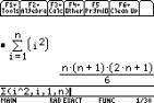
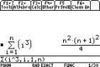
The summation function F3 4: S( sum will also give the general summation results in Theorem
4.2.1.
|
|
|
|
|
4.4 Fundamental Theorem of the Calculus
|
Instructions
|
Screen Shots
|
|
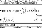
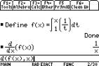
The derivatives of the integral functions
can be found on the TI-89 by defining the function first using F4 1: Define,
and then finding its derivative with respect to x (or these two steps can be done together).
|
|
|
|

|
|
|
|
|
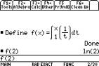
Using CAS with the theorem can help us
with antiderivatives for functions such as  . .
|
|
|
Areas under curves are best calculated by
evaluating the correct definite integral. This can be done numerically on the
graph screen, or on the " screen. For example to find the
definite integral  we can use the
graph of f(x) on the TI-89 to see the
area represented by the integral and numeric integration to calculate it. we can use the
graph of f(x) on the TI-89 to see the
area represented by the integral and numeric integration to calculate it.
• # x ´
2 ∏
• % F5 m 2
∏ 5
∏
|
|
|
Note : Only the x value of the lower and upper limit needs to be typed
in. Ignore the y-value. This should appear on your screen.
|
|
|
|
|
|
|
|
|
|
|
|
|
|
|
On the " screen we just
enter the function into F3 2:ò
integrate, and the lower and upper limits. Note the use of • ∏ again
(approximate mode) to get the decimal answer.
|

|
|
|
|
Area between the graphs of two functions
f and g.
Area =  , where x=a and x=b are the x-values of the two points
of intersection (if they exist).
, where x=a and x=b are the x-values of the two points
of intersection (if they exist).
We can also use the formula  to find the area
between the graph of f and the x-axis, and then we do not have to worry about where the
function intersects the axis or the signs of the integrals. This works well on
the TI-89 since we have the function abs.
to find the area
between the graph of f and the x-axis, and then we do not have to worry about where the
function intersects the axis or the signs of the integrals. This works well on
the TI-89 since we have the function abs.
For example calculate
the area between f(x)= and the x-axis from x=–1 to x=2. It is always good to look
at the graph of the function to see what is going on.
and the x-axis from x=–1 to x=2. It is always good to look
at the graph of the function to see what is going on.
|
Instructions
|
Screen Shot
|
|
Define y1
= x(x + 1)(x –2) and draw the graph. Entering y2
as abs(y1(x))
(which gives a reflection of y1 in the x-axis) enables the area to be found without finding the
intersections with the axis. Note that the area is NOT equal to  (compare
screens 2 and 4) (compare
screens 2 and 4)
|
|
|
|
|
|
|
|
|
|
|
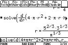
5. Integration
techniques
|
Instructions
|
Screen Shot
|
|
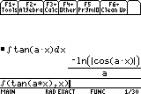
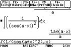
Specific techniques for integration are
not required when using the TI-89 since it will integrate all integrable
functions, using the ∫ function. However, we can verify some of the formulas
for general results, as well as more specific functions.
|
|
|
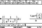
Note how functions such as  are entered,
and the need for ( ) around the whole of a numerator and/or a denominator in are entered,
and the need for ( ) around the whole of a numerator and/or a denominator in  and and  . .
|
|
|
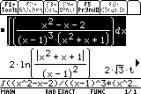
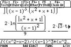
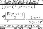
Integrating a rational function
|

|
|
An inverse trig function.
|
|
|
Integrating a rational function
|
|
|
|
|
|
|
|
|
Indefinite and definite integrals.
|
|
6 Functions of
Two Variables
|
Instructions
|
Screen Shot
|
|
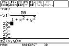
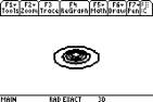
Set the graph drawing mode to 3D using
MODE Graph 5: 3D. In the • Y= mode the
DEs are then set up ready for you to enter z1=
etc. The TI-89 uses y and x for these functions.
|
|
|
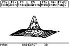
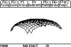
Use • [GRAPH] to draw
the graph (this may take a few seconds)
You may need to resize the window using • [WINDOW]
where you can set all three variables. The viewing angle can also be changed
using the eye variables or by using the  keys. keys.
|
|
|
Pressing [ENTER] will rotate the graph dynamically.
|
|
|
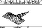
We can draw contours too.
Select the • Y= mode and
press • |
Change Style 1: WIRE FRAME to 3: CONTOUR LEVELS and
press ∏. Use • [GRAPH] and then F6 Draw 7: Draw
Contour command in the graph mode to enter the x and y values (here each 0). This
can also be rotated discretely or dynamically.
|
 ( (
|
|
Here is the graph of  . .
|
|
|
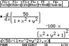
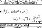
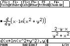
For partial derivatives, the TI-89
assumes letters to be constants unless told they are variables, so will do
these as shown using F3 1: d( differentiate
Here with respect to x
|
|
|
Here differentiate with respect to x…
|
|
|
…and here with respect to y
Remember that these are the partial
derivatives fx(x,y) and fy(x,y) not what the CAS notation implies.
|
|
|
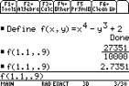
We can use the F4 1: Define to define a
function in two variables and hence find the value of the function.
|
|
|
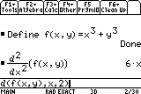
We can get fxx by differentiating
twice with respect to x…
|
|
|
…and fyy by differentiating
twice with respect to y
|

|
|
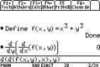
For fyx and fxy we differentiate
twice, once for each variable.
|
|
|
|
|
|
Example 207
|
|
|
Then use the Hessian obtained as above to
test each point.
|
|
7 Linear Systems
7.1 Gaussian
Elimination
Matrix notation
This can be done using the row operations
on the TI–89, or using functions which give echelon form and reduced echelon
form. First, we need to know how to enter a matrix into the Data/matrix Editor
or into the Home screen.
|
References: TI-89
Guidebook 229-233
|
|
Instructions
|
Screen Shot
|
|
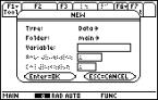
Press O 6, open the Data/matrix editor and then select 3.
New
|
|
|
For Type,
select Matrix, as following.
|
|
|
Press B and select 2: Matrix.
|
|
|
Press D D and enter the variable name M1. (Some
names are reserved, if you try to use a reserved name you will get an ERROR
message).
Enter the row and column dimensions of
the matrix.
|
|
|
Type in the first three rows and columns
of the matrix. You will need to use the arrow keys to move around. Press
ENTER to register each entry. You can use fractions and operations when you
enter values.
|
|
|
Press the " key and enter M1
return. You should now see the matrix in this standard form.
|
|
Entering a matrix into the Home Screen
|
Instructions
|
Screen Shot
|
|
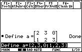
Method 1:
From the Home screen, enter a matrix by
using Define(which can be accessed by F4 1 or
could be typed in). Use the square bracket [ ] to enclose the matrix. We
enter the matrix by typing the first row and then the second and so on. Use
commas to separate entries and semicolons to separate rows.
|
|
|
Method 2:
To enter a matrix into the Home screen,
use one set of brackets around the entire matrix and one set of brackets
around each row. Use commas to separate the entries in a row. Then press STO®, type a name for the matrix, and press ENTER.
Example:
[[1,2,3][-1,3,4]] STO® r ENTER
|
|
7.2 Matrix Row Operations
|
Instructions
|
Screen Shot
|
|
To swap two rows in one matrix, use 2nd
[MATH] 4:Matrix J:Row ops 1:rowSwap(.
|
|
|
Example:
We can change rows 1 and 2 of matrix
r with the command rowSwap(r,1,2).
|
|
|
To add the entries of one to those of
another row, use 2nd [MATH] 4:Matrix J:Row ops 2:rowadd(.
Example: Add
the entries of row 1 to those of row 2 and store them into row 2 with the
command rowAdd(r,1,2).
|
|
|
To multiply the entries of one row by a
value, use 2nd [MATH] 4:Matrix J:Row ops 3:mRow(.
Example:
Multiply the entries of row 1 by 3 and store
them into row 1 with the command
mRow(3,r,1).
|
|
|
To multiply the entries of one row by a
value and add the products to another row, use 2nd [MATH] 4:Matrix J:Row
ops 4:mRowAdd(.
Example:
Multiply the elements of row 1 by 3, add the products to row 2, and store
them into row 2 with the command mRowAdd(3,r,1,2).
|

|
Example 7.2.2:
|
Instructions
|
Screen Shot
|
|
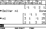
First enter the augmented matrix, here into m1.
Note: To
remove a variable used for a matrix or other calculation use
Ω Delvar (variable name).
|
|
|
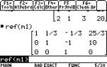
Then use the command I menu (2 5) select
4: Matrix and 3. ref for row echelon form,
|
|
|
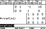
or 4. rref for reduced echelon form.
|
|
7.3 Systems which contain unknown coefficients
Example
7.3.1:
For what values of k does the following system of linear equations have no solution, a
unique solution, or infinitely many solutions?
x1
– x2 + x3 = 2
3x1
+ x2 – x3 = 2
2x1
+ x2 – x3 = k
|
Instructions
|
Screen
Shots
|
|
First enter the augmented matrix, here into m, then
continue as follows:
|
|
|
R2 –3R1®R2
mRowAdd(–3, M, 1, 2) ß M
multiply R1 by –3, add the product to R2
and store it in row 2.
|
|
R3-2R1®R3
mRowAdd(–2, M, 1, 3) ß M
multiply R1 by –2, add the product to R3
and store it in R3.
|
|
|
¼ R2
mRow(1/4, M, 2) ß M
multiply R2 by ¼
|
|
|
R1+R2®R1
rowAdd(M, 2, 1) ß M
add R1 to R2 and store it in R1.
|
|
|
R3-3R2®R3
mRowAdd(–3, M, 2, 3) ß M
multiply R2 by –3, add the product to R3, store it in R3.
|

|
Of course we can get the last stage
directly using rref(m). However,
note that the full working
will be required
for the examination.
We see that the coefficients of the
variables have all become zero on the bottom row, R3, so we can not have a
unique solution.
Thus if k –
1 = 0 i.e k = 1 then there will be an infinite
number of solutions.
If k≠1 then
we get an inconsistent set of equations since R3 is false and there are no
solutions. There is never a unique solution.
When k = 1 x2
– x3 = –1 so x2 = x3
– 1
and x1
= 1
so for any real number parameter t
(x1, x2, x3) = (1, t – 1, t) a straight line.
8. Matrices
8.1 Matrix arithmetic
|
Instruction
|
Screen Shot
|
|
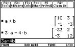
|
|
|
|
|
|
|
|
|
|
|
|
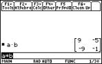
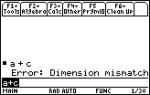
To perform
matrix arithmetic simply
define the matrices.
|
|
|
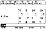
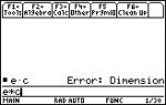
Then find
the sum or the difference.
|
|
8.2 Multiplying matrices
8.3 Identity Matrix
|
Instructions
|
Screen Shot
|
|
Identity
matrix
This is
defined as that matrix I for which
AI
= IA = A
|
|
|
|
|
|
On the TI-89 this is obtained by :
2 I {see 5} 4: Matrix
6: identity (
then type n) for an nxn identity.
|
|
|
|
|
|
Example:
|
|
8.4 The Transpose of a Matrix
|
Instructions
|
Screen Shot
|
|
On the TI-89 the transpose AT of a
matrix A is obtained by : [2, 3; –4, 2] ß a ∏ a 2 I 4: Matrix ˙ 1: T ∏
|
|
|
|
|
|
|

|
|
Example:
|
|
|
|
|
Example 8.4.1:
Consider the following matrices.
A= B=
B= C=
C=
D =  E =
E =
 F=
F=
If possible, compute each of the
following.
a)
A + B b)
3A - 4B
b)
3A - 4B c) A.B
d) A + C
e)
D.E
f) E.D
g) E.C
h)
D.E + F
Here are the results.
8.5 The inverse of a matrix
Example 8.5.1:
|
Instruction
|
Screen
Shot
|
|
To find the inverse of a matrix enter the
required matrix. The augmenting is done with the following commands:
|
|
|
2 I {see 5} 4: Matrix 7: augment( then 2 I {see 5} 4: Matrix
6: identity(
then type 3)) and store the result in A
using ß A.
|
|
|
We would then add –2 lots of row 1 to row
2 (R2+ (–2)xR1) and store the result in A using
2 I {see 5} 4: Matrix J: Row ops 4: mRowAdd(
mRowAdd(–2, A, 1, 2) ß A
|
|
|
Continue as above, remembering to edit
the last command each time to save time.
|

|
|
|
|
|
Here is the inverse of the matrix.
|
|
|
The TI-89
will give us the inverse of matrix A directly as follows, if it
exists.
j A ^ (-) 1
NB remember to use the (-) not the
minus sign!
|
|
8.6 Inverses and systems of Equations
|
Instructions
|
Screen Shot
|
|
Not all square matrices have an inverse
(such matrices are called singular). If we
try to obtain the inverse of a matrix
which is not invertible on the TI-89, an error results.
|
|
|
Solving systems of equations using
inverses. We can solve an equation of the form
AX = B
by multiplying both sides on the left by A–1
A–1AX
= A–1B
IX = A–1B
X = A–1B
So the solution comes from calculating
A–1B. Actually
this is not an efficient way to solve equations, but it is an alternative,
provided the inverse exists.
|

|
|
Using the TI-89 here we first enter the
matrix A and the vector B.
|
|
|
Then simply calculate A–1B.
|
|
Application
of systems of linear equations
Example 8.6.1:
A baby food is to be manufactured from the
ingredients carrot, cereal, and chicken. The amounts of three vitamins,
measured in mg per ounce are as shown below:
|
|
Vitamin
A
|
Thiamine
|
Riboflavin
|
|
Carrot
|
1
|
0.02
|
0.01
|
|
Cereal
|
0
|
0.10
|
0.05
|
|
Chicken
|
0
|
0.02
|
0.05
|
Calculate in what proportion these
ingredients should be mixed in order to produce a mixture with the three
vitamins in the ratio 5:4:3.
Solution:
|
Matrices
|
TI-89
|
|
In matrix form we have:
k>0,
and solving by row reduction to echelon form we use:
|
On the TI-89 this can be approached
directly, by multiplying by A–1. Note the K is put inside B.
|
|
Note we can actually work without the ks.
R2x100; R3x100

R2–2R1; R3–R1

|
|
|
R3«R2; R3–2R2; R2/5
R3/–8; R2–R3

so  and the required ratio is 5:34:25. and the required ratio is 5:34:25.
|
The required ratio is 5:34:25.
|
8.7 Determinants
|
Instructions
|
Screen Shots
|
|
The determinant of a 2´2 matrix is obtained on the TI-89 by :
2 I 4: Matrix ˙
2: det ([a, b ; c , d] d ∏
|
|
|
For example:
|
|
|
The
determinant of a 3´3
matrix is
obtained on
the TI-89 by :
[3, 2, –1 ;
1, 6, 3; 2, –4, 0] ß a ∏
2 I 4: Matrix ˙
2: det ( a d ∏
|
|
Determinant can be used at the start of
a problem on simultaneous equations to check for consistency.
Example 8.7.1:
Solve the following sets of simultaneous
equations.
|
Equations
|
|
|
a) x+y
= 4
2x+2y= 6
|
|
|
|
|
|
No Solution.
|
|
|
b) 2x- y = 3
4x-2y = 6
|
|
|
|
|
|
Infinitely many solutions.
|
|
|
c)
4x –
3y = 12
x – 2y = –2
|
|
|
|
|
|
Unique solution: x = 6 and y = 4
|
|
9. Vectors
9.1 Eigenvalues and Eigenvectors
Example 9.1.1:
Find the
eigenvalues and eigenvectors for the following matrices:
A= B=
B= C=
C= D=
D=
Solution:
|
Instructions
|
Screen
Shot
|
|
Use the define option to enter the
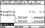
matrices as a, b, c, and d, respectively. To find the eigenvalues of the matrix A, use Math 4 9 a ) ENTER or type eigvl(a) and ENTER. To find the eigenvectors of the matrix a use Math 4 A a ) ENTER or type eigvc(a). The figure shows the eigenvalues and
eigenvectors of the matrix A.
|
|
|
Note: The first column of
the result of eigenvector is an eigenvector corresponding to the eigenvalue
which is listed in eigv1(a), similarly for the
second. Note that TI 89 is normalizing the vectors, that is the eigenvectors
are unit vectors. For easier
notations, it is convenient to rewrite the eigenvectors with integer entries. One possible method is to replace the
smallest number in the columns by 1 and divide the other entries in that
column by the smallest value you just replaced. Use the command eigvc(a)[j,k]
to refer to the j-k entry of the matrix eigvc(a). It is clear that the entries in the first column are equal. Thus
for an eigenvector corresponding to the eigenvalue -1, we may take  The second one
may not be clear so we replace -.316228 by 1. Note then that -.96683/-.316228
is 3.062. Thus it is highly recommended that you compute eigvc(a)[2,1]/
eigvc(a)[2,2]. We find that this is 3. Thus we
may take The second one
may not be clear so we replace -.316228 by 1. Note then that -.96683/-.316228
is 3.062. Thus it is highly recommended that you compute eigvc(a)[2,1]/
eigvc(a)[2,2]. We find that this is 3. Thus we
may take  as the second
eigenvector. as the second
eigenvector.
|
|
Instructions
|
Screen Shot
|
|
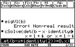
If we are evaluating eigvl(b), we will get the message Non-real result. This means that the characteristic equation of the matrix B has complex roots. Note that by using the command cSolve(det( b – x*identity(2))=0,x) ENTER, we get the complex eigenvalues, namely, x=1+i or
x=1-i
as shown.
|
|