Matlab MCMC
solver code by Dr. Fox
Matlab PDE
solver code by Dr. Fox
Week of 21st November 2005:
We began our summer
scholarship. We ran into trouble acquiring a computer in the Maths
department to use, so Dr. Fox allowed us to use his personal computer.
We began by installing Python on this and began learning the language.
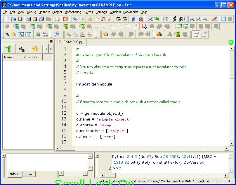
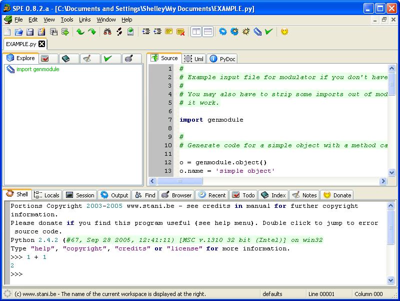
During this week we also installed various IDEs, including Eric and
SPE,
to test their performance and usability. We found them to be
unsatisfactory, as they seemed buggy and complex to use. Most also
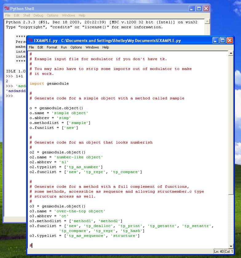
required Python 2.4. We decided to
use the simpler
IDE included with
Python, IDLE. We also ran into trouble trying to get a working version
of SciPy
installed, as at the time there was only a complete version of SciPy
available for Python versions 2.3 and below, and only the core
functions were available for the latest version of Python, 2.4. Because
of this problem, we decided to use Python 2.3.
Week of 28th November 2005:
We received the
original Matlab code from Dr. Fox and he gave us an
overview of what each part of the code did. We started implementing the
more simpler functions in Python, such as PickN and ChooseNFromM. Later
in the week we began to implement the MakeData function, which contains
most of the information about the resistor
network, as a
class in Python, to allow use to access the data more
conveniently. We encountered problems implementing sparse
matrices and other SciPy
functions in python, as these functions appeared to have been converted
directly from Fortran and consequently were completely undocumented in
the SciPy package. We eventually managed to implement all of the
functionality in
MakeData, but found that the code took around 10 seconds to run rather
than around 2 seconds for Matlab. We managed to optimise the code by
fiddling around with sparse matrix code.
Week of 5th December 2005:
We continued to work on MakeData, and managed to get the code running
at a satisfactory speed. With a working dataset, we began to work on
the main body of the code
and eventually got some code that would run through the whole loop (but
which habitually crashed).
However, each iteration took around 2 seconds to complete, much slower
than the Matlab code, which could run a couple of iterations per
second. We accidentally erased all of our function code because of a
bug in IDLE,
but were able to use a Python
decompiler to retrieve the code from the .pyc files that were left,
but not after having to bring in a personal computer running Linux to
build the decompiler from source, as the Windows version
was not available for free.
Week of 12th December 2005:
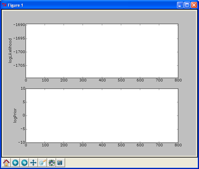
We started writing PlotStats function, and decided to use matplotlib
for output, as it claimed to emulate Matlab style commands well. Here
is an example of the plot created.
We continued improving
plotting code, including splitting the
plotting code into two functions, one to create the plot and another to
update it. We encountered problems trying to get our statistics plot to
update in each loop, as we found that after the first graph had been
drawn the program would not continue running until this graph was
closed. According to the matplotlib documentation we were meant to be
using the matplotlib command show rather than draw, but neither command
seemed to work as we wanted. We eventually found that by using the
interactive mode of matplotlib, we were able to get our
statistics plot to not wait for user input. Our program was still
running very slowly. We investigated why our program took so long to go
through the main
loop, and found that the main source of delay was the Solver function.
To improve this, we could use permutations of the data set rather than
the full 625 x 625 set as Matlab did (using the symamd
function), but this function was only available in Matlab or as C code, and not in
Python. We tried to
implement Cholesky factorisation without these permutations, but found
that there was a bug in our code causing our reduced stiffness matrices
to sometimes be non-positive definite, and had problems creating test
functions to see what was causing this. We also began designing this
web page.
Week of 19th December 2005:
We
managed to find the source of our
crashes, as the R matrix we were creating was sometimes non-symmetric,
seemingly because of a transition from column to row format in the
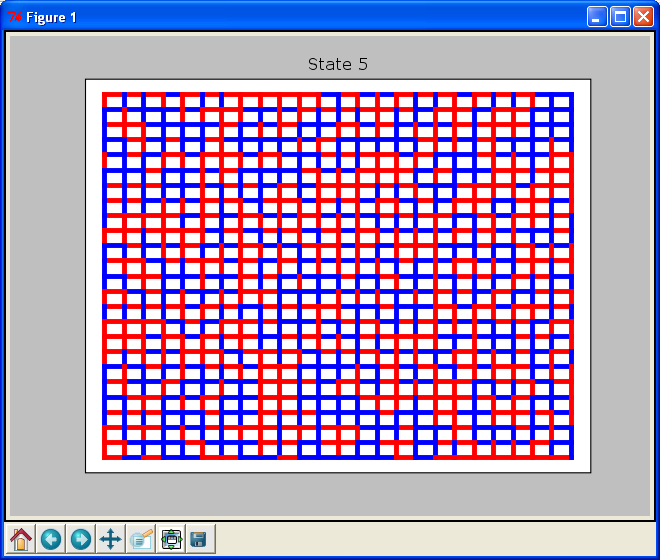
sparse matrix construct. We also began writing the code to display the
resistor network (and resistance values for each resistor). We managed
to create code to display the network (example),
but had the same problems with
show and draw as before, so the graph did not update very well. We then
began investigating what would need to be done to have the symamd
function available in Python for us to use, by implementing the C code
as a new Python module. We encountered problems
with this, as Python requires new modules to be compiled using the same
compiler as
for the main system. Under Windows, Python was compiled with Microsoft
Visual C++, which we did not have. Under Linux on the maths department
server, we did not have access to the python directory to add in our
compiled modules. Because of this, we decided to concentrate on fixing
bugs in the current code, and not use the symamd function.
Break 22th December 2005 -
5th February 2006
Week of 6th February 2006
We
continued to work on fixing bugs in our current code, but also began
working on the partial differential equation solver for the resistor
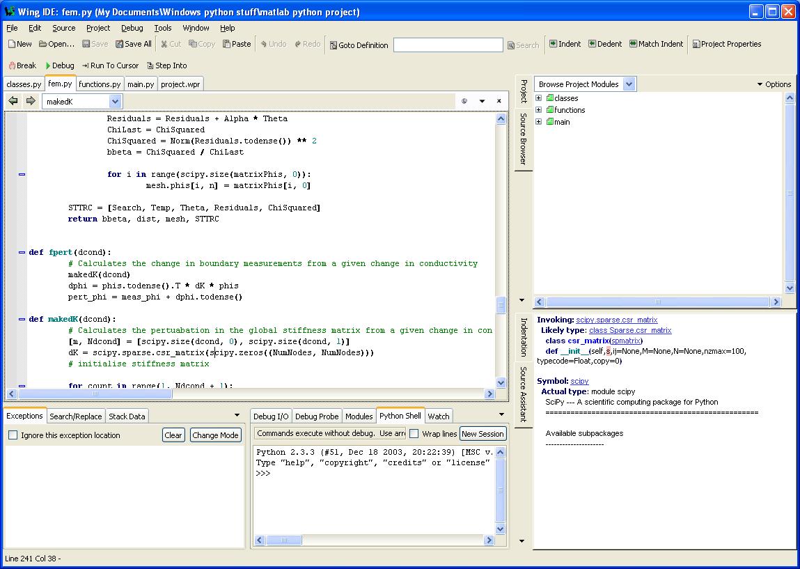
network at the request of Dr. Fox. We also began testing Wing IDE after
this was acquired for us by Dr. Fox, and found this very easy to use,
and helpful with our coding, as it provided advanced debug facilities
which aided in finding many bugs in our code. For example, we managed
to fix a major bug
in our Solver code in the MCMC version which was causing incorrect
Green's functions to be
calculated, by being able to check the value of the Green's functions
at various places in our code. However, even once we fixed this, there
still appeared to be a bug in the code causing the DR matrix not to be
updated correctly, even though there appeared to be differences between
the old and new proposals from our tests. It could possibly be related
to the slowness of our code, in that the code did not loop enough times
to update the DR matrix.
Week of 13th February 2006
We continued work on
the partial differential equation code, rewriting the program to not
use global variables at the request of Dr. Fox. This required some work
in creating a more functionally oriented structure for it, and working
out which variables were needed in the various scopes. We managed to
easily create the dataset we needed in the SetMesh function, but had
more problems creating the looping code needed in the fsolve function,
because of various issues with variable scope and sparse matrices. As
SciPy does not have some Matlab functions used in our code, we had to
write code to emulate these functions, such as norm and meshgrid. We
eventually managed to create code that would run through a few
iterations, but it seemed that our code only took around half the
iterations of the Matlab code to update the potential, suggesting a
problem. The code also seemed to periodically enter an infinite loop,
for reasons we were unable to determine.
Week of 20th
February 2006
A new version of SciPy was released, which seems to
address some of the
issues we encountered when trying to implement our program. However,
the newer version is not completely backwards compatible, so our code
will require some rewriting to work with it. As we only had one week
left, we decided not to work on changing the program to work with SciPy
0.4.6. Because of time constraints we focused on completing our report
and conclusions, and
documenting the code, over continuing to work on debugging it. While
all of the Matlab code had been converted to Python, there are some
bugs related to the transfer that we had been unable to debug in the
time we had.
Conclusions
We
have decided that while Python is
a better solution for developing
programs, Matlab is presently better for scientific computing tasks.
Matlab has benefit of being a thoroughly documented and integrated
solution, with no need to install a number of different packages from
different sources, while still remaining extensible. Although there are
integrated Python solutions such as Enthought's version of Python,
these do not include all packages needed, and are currently very out of
date. While documentation for Python itself is complete and easily
available, SciPy is currently scarcely documented, and some parts of
the functionality such as sparse matrices are simply not documented at
all, making it much harder to begin creating code for it. Also, it is
much easier to find function help in Matlab, as it simply requires
typing "help function", while in Python searching for function help is
harder as you need to know which Scipy package the function you
are looking for is in. While Matlab
and Python have a similar syntax, there are very many differences and
incompatibilities between them that made transferring code from Python
to Matlab difficult. For example:
- Indices
in Matlab start from 1,
whereas in Python they start from
0.
- Matlab
allows you to pass lists and
matrices as indices to
matrices, but SciPy did not support this at all in the version we used,
and the newer version does not implement it in the same way that Matlab
does. To implement the Matlab style, we had to write our own function
(which took time to create and was not very efficient)
- Many
common Matlab functions such as
converting from indices to
subscripts and vice-versa, calculating norms and retrieving a list of
non-zero entries from a sparse matrix were simply not implemented in
Python or
SciPy, meaning we had to write our own versions of these functions,
with implications for the speed of the program.
- Many SciPy constructs such as sparse
matrices did not seem fully
completed, as they did not support simple functions like transposes or
comparisons. This meant we had to convert between dense and sparse
matrices within the code, affecting the speed of it.
- Matlab supports various syntax
constructs such as "1:2:11" to construct a list, while these are
implemented as functions in Python ("range(1, 11 + 1, 2)"). Python also
does not implement these in the same way as seen in the example.
In conclusion, while SciPy
appears to have all the required functionality to implement various
mathematical tasks, simply converting Matlab code to Python code is
difficult because of the differences between the languages. SciPy also
suffers from still being heavily in development, meaning that some
functionality is not sufficiently documented or in some case not
implemented fully. Possibly once SciPy reaches version 1.0 and some
stablisation of the code and functionality has been achieved, it will
be a suitable replacement for most mathematical tasks that currently
use Matlab. The code we created in Python seemed much slower than the
Matlab code, though this could be attributed as much to problems with
our programming style and lack of time to streamline the code as much
as a genuine speed difference between the two.
Programs used
Python versions used:
2.3.5, 2.4.2
Python packages installed
Numeric 23.5
SciPy 0.3.2, 0.4.6
matplotlib 0.85, 0.86.2
IPython 0.6.15, 0.7.1
IDEs tested (screenshots):
Eric 3 (2005-04-10)
IDLE 1.0.2
SPE
0.7.5
Wing IDE 2.0.3-1
Links
Programs
IDEs
Documentation:
Programs to install to run code (under Windows)
Uses the latest version of
the various programs available unless the
latest version is incompatible.
- Install Python
2.3.5
- Install Python
win32 extensions build 207 (sourceforge link)
- Install Numeric
23.5 (sourceforge link)
- Install SciPy 0.3.2
- Install IPython
0.7.1
- Install ctypes
0.9.9.3 (sourceforge link)
- Install readline
1.12 (sourceforge link)
- Install matplotlib
0.86.2 (sourceforge link)
Or install Enthought's version
of Python, and skip steps 1, 3 and 5.
Steps 5-7 are only needed if you
want to use IPython, and are not
required to run our code.
Newest version of SciPy
instructions (our code will need slight
revisions to work with these):
- Install Python
2.4.2
- Install Python
win32 extensions build 207 (sourceforge link)
- Install NumPy
0.9.5 (sourceforge link)
- Install SciPy 0.4.6
- SSE1
(sourceforge link)
- SSE2
(sourceforge link)
- Install IPython
0.7.1
- Install ctypes
0.9.9.3 (sourceforge link)
- Install readline
1.12 (sourceforge link)
- Install matplotlib
0.86.2 (sourceforge link)
Last updated 24/2/2006