 Return
to Genesis of Eden?
Return
to Genesis of Eden?Fractal and Chaotic Dynamics
in Nervous Systems
Chris C. King Mathematics Department, University of Auckland.
1991 Progress in Neurobiology 36 279-308
Abstract : This paper presents a review of fractal and chaotic dynamics in nervous systems and the brain, exploring mathematical chaos and its relation to processes, from the neurosystems level down to the molecular level of the ion channel. It includes a discussion of parallel distributed processing models and their relation to chaos and overviews reasons why chaotic and fractal dynamics may be of functional utility in central nervous cognitive processes. Recent models of chaotic pattern discrimination and the chaotic electroencephalogram are considered. A novel hypothesis is proposed concerning chaotic dynamics and the interface with the quantum domain.
Contents :
This review surveys fractal and chaotic processes in brain dynamics and provides workers in experimental fields with a compact source of material in mathematical chaotic dynamics as a reference. An attempt has been made to make the mathematical aspects of the paper remain approachable to a variety of readers. Full background references are given to enable the reader to gain further in-depth treatment, and to explore more fully the variety of specialist topics leading out from the discussion.
Section 1 provides a compact mathematical introduction to fractal and chaotic dynamics. Most of the systems discussed here have specific application to experimental results in later sections. Sections 2 and 3 complement this with source material on mathematical modelling of neural nets and on biological neurons. In section 4 chaos at the cellular level is discussed, including models of the excitable membrane and ion channel. In section 5 chaotic neurosystems models and experimental results are considered including the Freeman-Skarda model and studies of the EEG. Section 6 touches on issues connecting quantum chaos, causality and the mind.
The aim of the review is to make it possible for a reader to gain a comprehensive overview of chaos as it applies to neural processes, to compare chaotic models with their alternatives and to assess the scope of chaotic and fractal processes in the conceptualization of the physical basis of brain function.
1: Concepts and Techniques in Chaos
(a) Chaotic systems This introduction provides a general description of chaotic dynamics and outlines techniques useful in analysis of experimental results.
A dynamical system is defined to be a set of first-order differential equations :
![]() [1.1]
[1.1]
The system is called autonomous if ![]() , i.e. the functions are not changing
with time. Systems of higher-order differential equations can be reduced
to first-order systems by a suitable change of variables. For example the
equation of harmonic motion
, i.e. the functions are not changing
with time. Systems of higher-order differential equations can be reduced
to first-order systems by a suitable change of variables. For example the
equation of harmonic motion ![]() can be simply reduced to the system
can be simply reduced to the system ![]() . This
type of formulation is general to Hamilton representations of conservative
energetic systems, (see [2.2]).
. This
type of formulation is general to Hamilton representations of conservative
energetic systems, (see [2.2]).
A dynamical system is generally defined on a configuration space consisting
of a topological manifold. A manifold is locally like Euclidean space![]() , but
may have varied global structures, as exemplified by the cylinder, torus,
fig 5(a), Klein bottle and other higher-dimensional spaces.
, but
may have varied global structures, as exemplified by the cylinder, torus,
fig 5(a), Klein bottle and other higher-dimensional spaces.
Integration of the equations [1.1] to ![]() [1.2]
[1.2]
yields integral curves or trajectories forming a flow on the manifold. The sets of these flow curves are called orbits. The flow thus integrates the field of velocity vectors determined by [1.1].
Linear differential equations admit analytic solutions and have well-defined
asymptotic behavior as ![]() , converging to fixed points, or periodic oscillations,
forming closed orbits. By contrast, even the simplest deviations from linearity,
including quadratic, bilinear and piecewise-linear functions can, under
suitable conditions, result in more complex chaotic behavior, in which the
orbits of the system are attracted to a complex higher-dimensional subset
called a strange attractor, or are ergodic. Ergodic flows behave like thermodynamic
systems in that they can be modelled over statistical ensembles because
the orbit fills a (possibly dense) set of invariant measure.
, converging to fixed points, or periodic oscillations,
forming closed orbits. By contrast, even the simplest deviations from linearity,
including quadratic, bilinear and piecewise-linear functions can, under
suitable conditions, result in more complex chaotic behavior, in which the
orbits of the system are attracted to a complex higher-dimensional subset
called a strange attractor, or are ergodic. Ergodic flows behave like thermodynamic
systems in that they can be modelled over statistical ensembles because
the orbit fills a (possibly dense) set of invariant measure.
An attractor is a subset of the manifold to which an open subset of points, the basin of the attractor, tends in limit with increasing time. For example in fig 1(b) for v = +1 the system has an attractor consisting of the closed circular orbit, with basins outlined by the arrowed flows. Existence of an attractor requires local volume to contract with increasing time and is consistent with a dissipative system in position-momentum representation. While conservative systems thus do not have attractors, they may still display classical chaos, see section 1(c)(iii).
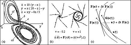
Fig 1 : (a) The Lorentz system displays sensitive dependence
in which neighboring trajectories separate exponentially with time. Neighboring
trajectories emanating from a are visibly separate by b and diverge into
distinct spirals by c1 and c2, so that their subsequent dynamics is unrelated.
(b) The Hopf bifurcation forms a periodic closed orbit attractor. For v < 0
there is only a sink (attractor). As v crosses 0 an attracting periodic
orbit and source (repellor) are created. The basins are indicated by the
arrows. (c) Geometric profile of the improved Euler method [1.4].
The hall-mark of a chaotic flow is sensitive dependence on initial conditions (Schuster 1986). Points which are arbitrarily close initially become exponentially further apart with increasing time, leading to the amplification of very small perturbations into global uncertainties. Sensitivity results in both an entropy increase associated with the loss of positional information with time, and in structural instability in which an arbitrarily small perturbation of the flow causes structural changes to the topology of the orbits ( although they may have similar qualitative behavior ). This prevents accurate long-term numerical approximation of the system with increasing time. In fig 1(a) sensitive dependence is illustrated. Neighboring trajectories emanating from a are visibly separate by b and diverge into distinct spirals by c1 and c2, so that their subsequent dynamics is unrelated. Note that each orbit has a unique winding sequence e.g. 1, 6, 3, 4, ... representing the number of times it negotiates each spiral arm of the attractor. An arbitrarily small perturbation will disrupt the winding sequence and hence change the topology of the orbits. The entropy results in a loss of memory of the initial conditions in any numerical approximation over time. The initial conditions thus cannot be retrieved by reverse iteration of the flow.
Time-dependent systems are capable of abrupt changes in their topological form called bifurcations as the underlying parameters cross critical values. Bifurcations result in abrupt catastrophic change in the topology of the flow under continuous variation of the time-dependent parameters. In fig 1(b) the Hopf bifurcation results in the formation of a closed orbit attractor (oscillation) from a point attractor (sink) at the origin as v crosses 0, see section 1(c)(ii). In fig 4(a) repeated pitchfork bifurcations result in subdivision of the logistic attractor, and the tangent bifurcation results in intermittent chaos, section 1(c)(i).
Because non-linear differential equations cannot in general be integrated directly, it is often necessary to resort to techniques of numerical integration in which a discrete transfer function is constructed which approximates a stroboscopic representation of the flow at discrete time intervals
![]() [1.3]
[1.3]
by using numerical methods such as the improved Euler method [1.4] or Runge-Kutta (Butcher 1987) :
![]() [1.4]
[1.4]
In a time-varying system, chaos may become established by three principal routes involving a (possibly infinite) sequence of bifurcations of the attractor, intermittent disruption of a periodicity, or the topological breakup of a surface, such as a torus, representing several linked oscillations. We will examine each of these three routes, because a knowledge of all of them is essential in characterizing chaotic dynamics in the brain and excitable cells.
A series of techniques have been developed for analysing chaotic systems which both lead to a conceptual understanding of their phenomenology and also provide methods for handling experimental investigations. These are outlined in the following sections.
(i) Liapunov Exponent and Entropy. Two of the most important attributes of chaotic systems are sensitive dependence on initial conditions and the loss of spatial information with time, resulting in an entropy.
In a flow with sensitive dependence the distance between adjacent points becomes exponentially further apart with increasing time. Repeated iteration of the corresponding chaotic map similarly causes the separation of two adjacent points to become exponentially increased. This provides a means of calculating the exponent of growth, called the Liapunov exponent.
Consider the repeated action of the discrete map ![]() increasing separation
by a factor
increasing separation
by a factor ![]() :
: ![]()
Hence we can write ![]() .
.
If the separation varies along the path, we can take limits as ![]() we
have
we
have
![]() [1.5]
[1.5]
![]() [1.6]
[1.6]
This formula makes it easy to calculate the Liapunov exponent for any iteration. In a chaotic system in one or more variables, sensitive dependence requires at least one of the Liapunov exponents to be greater than 1, thus resulting in exponential separation of trajectories.
Note that in the case of a continuous flow, the role of the constant a is slightly different.
In the flow ![]() , [1.7a] whereas with the map,
, [1.7a] whereas with the map, ![]() [1.7b]
[1.7b]
The formula [1.6] also naturally represents the loss of information, or entropy :
The Shannon informational entropy is ![]() [1.8]
[1.8]
where ![]() is the probability of being in state i and
is the probability of being in state i and ![]() .
.
Consider a single iteration in which [0,1] maps to [0,1] under separation
a.. At the initial stage, we have n states each with probability![]() , so
:
, so
: ![]() [1.9]
[1.9]
After one iteration, the resolution is reduced by factor ![]() , following the
same reasoning as in [1.6] for one step, giving
, following the
same reasoning as in [1.6] for one step, giving ![]() states each with probability
states each with probability
![]() ,
,
so we have : ![]() [1.10]
[1.10]
Thus there is thus a difference ![]() .
.
Averaging this over many iterations, we have ![]() [1.11]
[1.11]
which is obviously the same as [1.6] except for a factor of log 2.
For a 1-dimensional map we thus define the Kolmogorov entropy to be K = l.
When we have a higher-dimensional mapping or flow, there is an exponent
li for each dimension i in the configuration space. If the system has an
attracting set, volume contraction will cause the sum of the exponents to
be negative, thus allowing only some to be positive. Only the positive (expanding)
Liapunov exponents contribute to the spreading and so K is generally identified
with the sum of these positive exponents: ![]() [1.12]
[1.12]
A system with more than one positive exponent is referred to as hyperchaotic (Rössler 1979,1988).
From another point of view, the entropy may be associated with new information entering the system and over time replacing that associated with the initial conditions.
(ii) Power Spectrum. To distinguish
between chaotic and multiply periodic systems one can examine the Fourier
transform ![]() [1.13]
[1.13]
which transforms the function x(t) into a spectrum x(w) of frequency components, which for periodic motion consists of discrete frequencies, but for chaotic motion has a broad band spread.
The power spectrum squares the Fourier amplitudes to give positive real values
![]() [1.14]
[1.14]
In the case of a discrete iteration of finite length, such as a 2n cycle,
we can use a discrete transform to resolve the iteration into its Fourier
components ![]() [1.15]
[1.15]
This results for example in the 1024 step and 256 step Fast Fourier Transforms [FFTs] shown in fig 2(a). In (i) a 1024 point iteration of one component of the Lorentz iteration has been used to generate the discrete power spectrum using a Fast Fourier Transform [FFT] (Elliot et. al.. 1982). Although the flow has a strong periodicity its band-spread indicates chaos. (ii) The FFT of the self-similar Morse-Thule sequence (Schroeder 1986) 0110100101101001. . . This can be generated by recursive reflection of 01 in its complement [viz 01, 0110, 01101001, etc.], or by taking the binary digit sums of each positive integer mod 2, [viz 0 Æ 0, 1 Æ 1, 10 Æ 1, 11 Æ 0 etc.]. Although this is non-repeating, any discrete Fourier transform has a symmetric set of distinct components, as a result of symmetries in the self-similar structure.
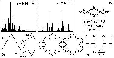
Fig 2 : (a) Power spectra (i) for the Lorentz system and (ii)
for the Morse-Thule sequence. Note the broad bandspread in (i) characteristic
of chaos despite the existence of a peak frequency. In (ii) although the
sequence is self-similar and non-periodic, the power spectrum consists of
symmetrical frequencies. (b) Koch flake formed by repeated tesselation of
a triangle and (c) Cantor set formed by repeated removal of the central
third of each interval are examples of fractals. (d) Julia set of complex
logistic map [1.24] for r = (3.4 + .02 i). This set is connected so that
points near zero iterate to a finite period attractor inside the set. Points
outside all iterate to infinity. Julia sets can also be disconnected, in
which case all other points iterate to infinity.
(iii) Hausdorff Dimension and Fractals. In a one-dimensional
set such as the interval [0,1], we need twice as many subsets of 1/2 the
length to cover the interval, 4 times as many of a 1/4 the length and so
on. In a two dimensional set, such as the unit square, we need ![]() times
as many 1/2 the length and so on. We can thus define the Hausdorff dimension
d as the exponent such that a covering by d-spheres of diameter
times
as many 1/2 the length and so on. We can thus define the Hausdorff dimension
d as the exponent such that a covering by d-spheres of diameter ![]() satisfies
, as
satisfies
, as ![]() [1.16]
[1.16]
A set is called a fractal if its Hausdorff dimension exceeds its integral topological dimension, i.e. if the Hausdorff dimension is not an integer.
Fractals often possess self-similarity on a change of scale between parts
of the set and the whole. A fractal which is constructed by recursive development
in stages, enables exact calculation of the Hausdorff dimension from [1.16]
using two successive stages of length ![]() and
and ![]() : [1.17]
: [1.17]
For example in the Koch flake, fig 2(b) each side is repeatedly replaced
by 4 sides each 1/3 the length. This gives rise to a Hausdorff dimension
of ![]() in the limit, hence a fractal. The Cantor set, fig 2(c) is formed from
[0,1] by removing the open middle third [e.g.
in the limit, hence a fractal. The Cantor set, fig 2(c) is formed from
[0,1] by removing the open middle third [e.g. ![]() ] from each remaining
subinterval, leaving 2 sides of the length 1/3.
] from each remaining
subinterval, leaving 2 sides of the length 1/3.
It is thus a fractal with dimension ![]() . Note that the Cantor set is identifiable
with all base 3 numbers in [0,1] having only 0 & 2 as digits, e.g. 0.0220020.
. . and thus maps 11 onto the whole interval [0,1] by mapping e.g.
0.0220020
. Note that the Cantor set is identifiable
with all base 3 numbers in [0,1] having only 0 & 2 as digits, e.g. 0.0220020.
. . and thus maps 11 onto the whole interval [0,1] by mapping e.g.
0.0220020 ![]() 0.0110010. This occurs despite the removal of a set of measure
0.0110010. This occurs despite the removal of a set of measure![]() ,
equal to that of the whole interval [0,1]!
,
equal to that of the whole interval [0,1]!
The strange attractors of chaotic dynamics are generally fractals. A
finite non-integer dimension indicates that a dynamic is chaotic, rather
than stochastic. Iterations such as the logistic map [1.23] result in fractals
called Julia sets fig 2(d) , subsets which tend neither to a finite attractor
nor to infinity, but are mapped within themselves. They thus form the fractal
boundaries of the basins of attraction. The variety of Julia sets of the
quadratic mapping ![]() has been the subject of keen interest (Peitgen &
Richter 1986), as well as their relation to the Mandelbrot set fig 4(a).
The Julia set of each value r is a unique self-similar fractal each with
its own distinctive form. Given a connected Julia set, such as the one illustrated
in fig 2(d), for the period 2 region of the logistic map, points on the
interior basins all iterate to a finite attracting set, while those outside
iterate to infinity. The bounding Julia set consists of those chaotic points
which do neither. Such fractal basin boundaries appear to be general in
dynamical systems. Time-dependent systems may also generate fractal spatial
bifurcations to form dissipative structures enabling the generation of fractal
order out of chaos.
has been the subject of keen interest (Peitgen &
Richter 1986), as well as their relation to the Mandelbrot set fig 4(a).
The Julia set of each value r is a unique self-similar fractal each with
its own distinctive form. Given a connected Julia set, such as the one illustrated
in fig 2(d), for the period 2 region of the logistic map, points on the
interior basins all iterate to a finite attracting set, while those outside
iterate to infinity. The bounding Julia set consists of those chaotic points
which do neither. Such fractal basin boundaries appear to be general in
dynamical systems. Time-dependent systems may also generate fractal spatial
bifurcations to form dissipative structures enabling the generation of fractal
order out of chaos.
(iv) Correlation Integral: Generalized
Dimensions We can generalize the fractal dimension as follows (Grassberger
& Procaccia 1983, Roschke & Basar 1989). Consider a covering, as
above, with spheres of radius e, Pi the probability that a point falls into
sphere i, and ![]() the number of non-empty spheres. Then we define the
Réngi information of order q as :
the number of non-empty spheres. Then we define the
Réngi information of order q as :
![]() [1.18]
[1.18]
and the dimension ![]() [1.19]
[1.19]
Thus ![]() above; d1 & d2 are called the information & correlation dimensions.
above; d1 & d2 are called the information & correlation dimensions.
Grassberger & Procaccia (1983) formulated the correlation
dimension into a useful algorithm as follows :![]() [1.20]
[1.20]
where ![]() is the probability of points having distance
is the probability of points having distance ![]() , since each is the
probability
, since each is the
probability ![]() of
of ![]() being in the same
being in the same ![]() -sphere.
-sphere. ![]() can be calculated explicitly using
the Heaviside step function.
can be calculated explicitly using
the Heaviside step function.
![]() [1.21]
[1.21]
Since , we have ![]() [1.22]
[1.22]
making it possible to do a plot of log ![]() against log
against log![]() , to test for linearity,
fig 3(c).
, to test for linearity,
fig 3(c).
The correlation dimension is thus a more accessible measure of the dimension of a chaotic attractor than the fractal dimension, which is more difficult to calculate from a trajectory partly because the points do not become evenly spread on the attractor. Dimensions vary from 2.06 for the Lorentz attractor, through 4 for e.e.g. recordings of epileptic states through to values around 9 for a stochastic process with a small degree of correlation between the sample variables.
Because a long time series of vectors x1, ... , xn in the dynamic will have most of its variables uncorrelated because of exponential divergence of the trajectories, correlations between the variables will be a consequence of their lying on the attractor. Modifications of the Grassberger-Procaccia algorithm have been proposed (Theiler 1987, Albano et. al. 1988, Rapp et. al. 1989) which improve both speed and accuracy.
As a result of Taken's (1981) proof, a 1-D time series can be used to
form an embedding space for the attractor by taking k-vectors xit,
x(i+1)t, ... , x(i+k-1)t , by
taking a suitably large value for the dimension k. Increasing the time delay
t results in a saturation level tsat for a given k as the sampling time
becomes long enough to ensure non-correlation, fig 3(a). As k is increased,
tsat increases to a plateau, thus determining suitable k, t and hence d2
(Roschke & Basar 1989), fig 3(b). Various problems still remain. A suitable
choice of the window length (k-1)t and of the overall time epoch of the
sample must be made. A good measurement of d2 is made only if the slope
of the log-log plot remains say within a 10% variation over at least an
adjustment of a factor of 2 in e (Rapp et. al. 1989). A plot of the slope
against log e is useful here. The upper and lower bounds defining the region
should be indicated. One reasonable indicator of window length is to use
the autocorrelation function![]() [1.23]
[1.23]
to define the correlation time when the autocorrelation function has
fallen from 1 at t=0 to 1/ ![]() (Albano et.al. 1988).
(Albano et.al. 1988).
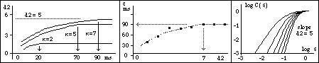
Fig 3 : The experimental determination of correlation dimensions
requires testing of parameters for saturation. (a) tsat versus k, as different embedding dimensions are used and the delay
k is increased, saturation occurs in the estimated dimension for different
delays. Adequate delay must be provided in each embedding dimension to get
a correct figure. (b) plateau in tsat at k = 7, illustrates that adequate
embedding dimension is also essential. (c) d2 from slopes of log C(e)-log
e plots has limit at k = 7. The dimensions are actually calculated from
the limiting slope of log C(e) against log e. Checks should be made both
that the parameters used do give linearity in the parameter range and that
they do converge to a good limit value.
A good plateau in the slope depends on a suitable window length a few times larger then the correlation time. Too short a window fails to provide a good plateau, on the other hand, making the window too large can result in the values no longer strictly adhering to a single trajectory and violating Taken's embedding theorem. Similarly care had to be taken with the time-epoch, which should be as long as possible but not long enough to result in non-stationarity in the phenomenon being measured. Researchers devising experimental tests for chaos are advised to consult Rapp (1989) before choosing their design and protocol. See also section 1(d).
It is also possible to measure the correlation dimension by taking a series of measurements from distinct spatial points in the dynamic, however this may result in a lowering of the measured value because the presentation of the attractor from the spatial sample is not fully unfolded (Babloyantz 1989).
(c) Iterations as Examples of Chaos
(i) The Logistic Map. Chaotic dynamics occur in some of the simplest iterative functions, including piecewise-linear and quadratic functions. To develop several aspects of chaotic behavior, we will examine a typical quadratic iteration, the logistic map :
![]() [1.24]
[1.24]
representing exponential population growth subject to a constrained area (Schuster 1986, Devaney & Keen 1989). The term r xn determines of exponential growth while the additional term (1 - xn) places a finite area constraint limiting the population.
It is easy to picture such an iteration in various ways. One is to successively evaluate the functions y = r x (1 - x) and x = y as shown in fig 4(bi). We pick an initial value x and evaluate y by moving vertically to the parabola. Next we let x = y by moving horizontally to the sloping line. The two steps combined result in one iteration i.e. xn+1 = y = r xn (1 - xn).
As the parameter r varies, the behavior of the iteration goes through a sequence of different stages. In (bi) the iterations are illustrated for r = 1 and 2 starting from two arbitrary points in [0,1]. Each iterates toward a fixed point, one at zero and the other positive. For the remaining figures the iteration is left to run for a few hundred steps, before plotting, so that only the limiting attractor is highlighted. Near the value 3.4 the iteration is attracted to a set of two values i.e. period 2, as depicted in (bii), in which the arrows still indicate the y = r x (1 - x) and x = y steps. At 3.56, (biii), the period 2 orbit has bifurcated twice to form a period 8 orbit. The effect of such period doubling is is clearly seen in the braided form of the attractor path. At 3.66, (biv), chaos has set in and the orbits now spread irregularly across the interval without returning exactly. At 3.8282 (bv) we are very close to the period 3 window. The period 3 iteration keeps slipping however, and intermittently enters chaos before returning to the attractor. At 3.8289 (bvi) period 3 has become stable. At 4.5 (c) the attractor has broken up and now most points escape to . A residual Cantor set of points (the Julia set) is mapped amongst itself, forming a Smale horseshoe (see section 1(c)(iii)).
Alternatively, we can plot all the x values that occur for a given r, once the system has been allowed to approach the attractor, as shown in fig 4(a). This gives rise to the attractor form diagram in which an initial point attractor repeatedly bifurcates into 2, 4, 8, ... values limiting in chaos at r, punctuated by further windows e.g. of period 3, and finally breakup of the attractor at r = 4.
Corresponding values of the Liapunov exponent are shown below this. For r < r, l < 0, reaching zero at each bifurcation point ri , but once chaos begins, l > 0, except for brief negative dips in the periodic windows.
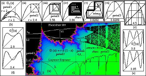
Fig 4 : The logistic map : The text contains a complete description
of all the phenomena in the diagram. (a) The forms of the attractor, Liapunov
exponent and Mandelbrot set, for 2.8 < r < 4 showing
the development of multiple period doublings, chaotic regions and periodic
windows. The attractor initially is a single curve (point attractor) but
then repeatedly subdivides (pitchfork bifurcations) finally entering chaos
(stippled band). Subsequently there are windows of period 3, 5 etc. with
abrupt transitions from and to chaos caused by intermittency and crises.
The Liapunov exponent![]() < 0 until chaos sets in. During
chaos it remains positive. The Mandelbrot set illustrates the fractal nature
of the periodic and chaotic regimes when x & r are extended to the complex
number plane. Complex number representation aids visualizing such fractal
structures. (b) A series of 2-D iterations of Gr(xn) including periods 1,
2 and 8 chaos, intermittency, and period 3. In (i) the two-step iteration
process is illustrated alternately evaluating y = r x (1 - x) (vertical)
and x = y (horizontal). As r crosses the value 1 a saddle-node bifurcation
occurs resulting in the attractor moving from zero and leaving a repellor
there (r = 2). In (ii) & (iii) period 2 and 8 attractors have formed.
In (iv) the iteration has become chaotic. In (v) the chaos is intermittently
entering a period 3 regime, which has become stable in (vi). (c) The Cantor
set of the horseshoe for r = 4.5. The attractor has now broken up resulting
in most points iterating to minus infinity, leaving only a Julia set of
exceptional points. (d) The pitchfork bifurcation illustrated. The double
iterate Gr^2(xn) twists to cross y = x an extra time, resulting in doubling
of the attractor into a period 2 set. (e) The tangent bifurcation illustrated
using the triple iterate Gr^3(xn). The lifting of the central tangent above
y = x removes the stability of period 3 causing slippage and intermittent
chaos.
< 0 until chaos sets in. During
chaos it remains positive. The Mandelbrot set illustrates the fractal nature
of the periodic and chaotic regimes when x & r are extended to the complex
number plane. Complex number representation aids visualizing such fractal
structures. (b) A series of 2-D iterations of Gr(xn) including periods 1,
2 and 8 chaos, intermittency, and period 3. In (i) the two-step iteration
process is illustrated alternately evaluating y = r x (1 - x) (vertical)
and x = y (horizontal). As r crosses the value 1 a saddle-node bifurcation
occurs resulting in the attractor moving from zero and leaving a repellor
there (r = 2). In (ii) & (iii) period 2 and 8 attractors have formed.
In (iv) the iteration has become chaotic. In (v) the chaos is intermittently
entering a period 3 regime, which has become stable in (vi). (c) The Cantor
set of the horseshoe for r = 4.5. The attractor has now broken up resulting
in most points iterating to minus infinity, leaving only a Julia set of
exceptional points. (d) The pitchfork bifurcation illustrated. The double
iterate Gr^2(xn) twists to cross y = x an extra time, resulting in doubling
of the attractor into a period 2 set. (e) The tangent bifurcation illustrated
using the triple iterate Gr^3(xn). The lifting of the central tangent above
y = x removes the stability of period 3 causing slippage and intermittent
chaos.
The sector of the Mandelbrot set of the logistic map fig 4(a) illustrates
the fractal nature of the envelope of iterates when both x and r have complex
number values. These enable us to visualize the fractal structures more
easily because they form a plane. Each r value in the Mandelbrot set gives
rise to a connected Julia set fig 2(d) and will hence iterate the central
value x = 1/2 to a finite attractor separated from infinity by the connected
Julia set (e.g. inside the Julia set of fig 2(d)). The complement of the
Mandelbrot set will iterate 1/2 to infinity. In fig 4(a) the Mandelbrot
set becomes vertically extensive only for r values whose real part has Liapunov
exponent ![]() < 0. For
< 0. For ![]() > 0 it is confined to the real line, extending
a thread to the value 4 with tiny islands showing for r values in the odd
period windows. The Mandelbrot set, and particularly its complement near
their boundary, is famous for the beauty of its color contour computer iterations.
It has been described as the most complex object in mathematics.
> 0 it is confined to the real line, extending
a thread to the value 4 with tiny islands showing for r values in the odd
period windows. The Mandelbrot set, and particularly its complement near
their boundary, is famous for the beauty of its color contour computer iterations.
It has been described as the most complex object in mathematics.
We will examine the variety of dynamical phenomena which occur in the Logistic map by looking qualitatively at six situations, each of which highlights a distinct feature of importance :
(1) Point attractors : When r = 0 the attractor is initially zero. As the parameter r is increased from 0, the quadratic rises and at 1 crosses the line y = x resulting in a saddle-node bifurcation in which a single attractor becomes a pair : an attractor and a repellor. In higher dimensional situations we would have a saddle, fig 6(c) and an attractor or repellor (node). The point attractor moves up to positive x, leaving a repellor at 0. Outside [0,1] the iteration tends to minus infinity. This situation is illustrated in fig 4(bi) where for the transitional value r = 1 the iteration is still attracted down and to the left to zero, while for r = 2, zero is a repellor and the intersection of the parabola with the line y = x is an attractor.
(2) Period doubling : At value r1 ~ 3 there is a bifurcation of the fixed
attractor into a period 2 attracting set, as illustrated in (bii). Successive
period doublings at r2 etc., (bii, iii) cause the attractor
to have a sequence of periods 2, 4, 8, ... , 2n. These arise from pitchfork
bifurcations as illustrated obviously in the forkings of attractor form
in (a). Here the graph of the two-step iterate Gr^2(x)
= Gr(Gr(x)) twists across y =
x to cause a doubling of the period. In this range the Liapunov exponent
![]() < 0, except at r1 , r2 , etc. where
< 0, except at r1 , r2 , etc. where ![]() = 0.
= 0.
Universality : In (a) are outlined the bifurcation values r1, r2, ..., r and the distances d1, d2, ...
where dn are the widths of the period 2^n attractors where they straddle the symmetrical value 1/2.
The values![]() [1.25]
[1.25]
are determined by the Feigenbaum numbers d = 4.669, and ![]() = 2.502. These
are universal to all functions with a quadratic maximum and thus appear
in a variety of systems from biology to astronomy (Stewart 1989).
= 2.502. These
are universal to all functions with a quadratic maximum and thus appear
in a variety of systems from biology to astronomy (Stewart 1989).
(3) Chaos : At the limit value r![]() the iteration becomes chaotic, (biv)
and
the iteration becomes chaotic, (biv)
and ![]() > 0. The trajectories now spread over the interval [0,1]. They do
not recur as there are no finite periodicities, but approach each possible
value arbitrarily closely given sufficient time. The iteration now has sensitive
dependence, e-close initial points becoming exponentially separated. Although
the orbits appear equally spread across the entire possible range of values,
the details of each are structurally unique. Complexity grammars (Auerbach
& Procaccia (1990) further analysis.
> 0. The trajectories now spread over the interval [0,1]. They do
not recur as there are no finite periodicities, but approach each possible
value arbitrarily closely given sufficient time. The iteration now has sensitive
dependence, e-close initial points becoming exponentially separated. Although
the orbits appear equally spread across the entire possible range of values,
the details of each are structurally unique. Complexity grammars (Auerbach
& Procaccia (1990) further analysis.
(4) Odd Period Windows : Intermittency and Crises There are a series of windows in the chaotic region where chaotic behavior is abruptly interrupted by new periodic regimes of periods 3, 5, etc., (bvi). These windows contain for example 3.2n bifurcation sequences similar to that of (2). As a result of Li & Yorke (1975), the existence of a period 3 attractor guarantees the existence of periods of all orders and uncountably many aperiodic orbits (chaos). By Sarkovski, the periods follow the causal sequence :
3 ![]() 5
5 ![]() 7 ... 2n.3
7 ... 2n.3 ![]() 2n.5
2n.5 ![]() ... 2^4
... 2^4 ![]() 2^3
2^3 ![]() 2^2
2^2 ![]() 2
2 ![]() 1, n = 1, 2,
3,...
1, n = 1, 2,
3,...
At the left-hand end of the period 3 window, a new type of bifurcation, the tangent bifurcation occurs, in which the 3-cycle becomes intermittently disrupted by chaotic bursts, (bv). Intermittent disruption of a periodic dynamic constitutes a second route to chaos distinct from period doubling in which only a single bifurcation is required for chaos. These constitute two of the three classical route to chaos. In fig 4(e) the source of the tangent bifurcation is illustrated. The tangent to Gr^3(x) crosses y = x as r is decreased allowing the escape of the period 3 iteration. Immediately upon bifurcation, the tangent (upper fig) is adjacent to y = x causing a slow slippage of the 3-cycle with irregular breakout into short episodes of chaos. Hence the term intermittency.
At the right-hand end of the period 3 window is another type of abrupt transition to chaos called a crisis that is caused by a collision between a point repellor and the fanning chaotic sub-bands of period 3 forming small triangles in fig 4(a). This causes the chaos to be repelled so that it spreads suddenly across all values again. The 3 repellors originate from the birth of period 3 in the tangent bifurcation at the other end of the window.
(5) Julia sets and Horseshoes : For each value of r there is a residual fractal Julia set of exceptional points which do not converge to the attractors, but are mapped instead among themselves. The Julia set for an r value of the complex logistic map in the period 2 region is illustrated in fig 2(d). Complex values assist the visualization of Julia sets because complex numbers form a planar image which we can see.
For r > 4 the finite attractor ceases to exist, since the
graph now goes outside the unit square, allowing points to iterate to minus
infinity, however a Cantor set of points remains, fig 4(c) which are mapped
among themselves indefinitely, once all the points which escape to -![]() in
one or more stages are removed. These form a Smale horseshoe as described
below, fig 6(b). This is in fact the Julia set of the mapping, which in
this case is not a connected set, because of the destruction of the finite
attractor's basin.
in
one or more stages are removed. These form a Smale horseshoe as described
below, fig 6(b). This is in fact the Julia set of the mapping, which in
this case is not a connected set, because of the destruction of the finite
attractor's basin.
(6) External noise : In the presence of external noise, the higher periods become lost, leaving noisy low periods and chaos. Noise thus can mask high period attractors and create the impression of chaos, see fig 7.
(ii) The Transition from Quasiperiodicity to Chaos. A third route to chaos arises from the development of multiple ( in particular three ) frequencies through repeated Hopf bifurcations as illustrated in fig 5(a).
The Hopf bifurcation creates an oscillation by the formation of a cyclic closed orbit as in fig 1(b). Here the vector field F expressed in terms of polar coordinates (r,q) has a constant rate of rotation, and a quadratic radial component dependent on v. For v < 0 the radial component is negative for all r and hence the origin is a sink (attractor). As v crosses 0 a positive radial component develpos. An attracting periodic closed orbit attractor (oscillation) is created, leaving a source (repellor) at the origin, as represented in 1(b) for the value v = 1.
The quasiperiodicity route is common in the development of turbulent
phenomena through oscillations. The first and second Hopf bifurcations introduce
two frequencies which can be realized as a flow on a 2-torus to which the
rest of the flow is attracted, fig 5(a). This can be conveniently studied
using a Poincare map :![]() [1.26]
[1.26]
which maps a cross-section C of a flow into itself in the neighborhood of a periodic orbit by following the flow until it intersects the cross section again, fig 5(c). This results in an iteration on the cross section C in which points are mapped to their positions one cycle later. This is sometimes called a phase portrait because the mapping arises from the effect of a phase shift in the oscillation on the closed orbit.
The Poincaré map of a two-dimensional flow on the torus with angular
frequencies ![]() and
and ![]() results in a rotation of the circular cross section by an angle
results in a rotation of the circular cross section by an angle ![]() . Adding
a small perturbation
. Adding
a small perturbation ![]() we get :
we get :![]() [1.27]
[1.27]
If ![]() is rational, i.e. a, b integer, the orbits are periodic and meet themselves
again, fig 5(b) after b cycles through C. However if W is irrational, the
orbits pass arbitrarily close but never meet, fig 5(c) and are called quasi-periodic.
Each orbit is then dense and ergodic on the whole torus.
is rational, i.e. a, b integer, the orbits are periodic and meet themselves
again, fig 5(b) after b cycles through C. However if W is irrational, the
orbits pass arbitrarily close but never meet, fig 5(c) and are called quasi-periodic.
Each orbit is then dense and ergodic on the whole torus.
Further bifurcation to form a third frequency will generally lead to collapse of the corresponding 3-torus to form a strange attractor. Like the intermittency route, this results in chaos after only a finite sequence of bifurcations. It differs from the other two however in the increase in the dimensionality of the attractor with each bifurcation.
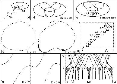
Fig 5 : (a) Repeated Hopf bifurcations result in tori. Creation
of two oscillations results in a flow on the 2-torus. (b) Periodic flow
on 2-torus results in closed orbits which meets themselves exactly. (c)
Poincare map of a cross section maps each point in a cross section C to
the corresponding point one cycle on along the flow. The flow illustrated
is irrational and hence has orbits consisting of lines which do not meet
themselves, but cover the torus ergodically passing arbitrarily close as
time increases. (d) Breakup of the torus under the circle map as K crosses
1. The increasing energy thus disrupts the periodic relationships as chaos
sets in. (e) f(q) versus q for the circle map. At K = .7 the function is
1 - 1 and hence invertible, but for K = 1.6 it is not. (f) The devils staircase
of mode-locked states. These order the possible rationals assigning to each
the interval of values for which such mode-locking occurs for K = 1. At
this value the mode-locked states fill the interval, leaving only a Cantor
set of irrational flows. (g) K - ![]() diagram of the circle
map showing mode-locked tongues (K<1) and chaos densely interwoven with
periodicity (K>1). The rational mode-locking exist only on the curves
for K > 1.
diagram of the circle
map showing mode-locked tongues (K<1) and chaos densely interwoven with
periodicity (K>1). The rational mode-locking exist only on the curves
for K > 1.
Study of this breakup can be facilitated by examining the dissipative
circle map derived from a periodically excited rotator (Schuster 1986):
![]() [1.28a]
[1.28a]
![]() [1.28b]
[1.28b]
In fig 5(d) is shown the cross section of the torus determined by this map and its breakup as K crosses 1.
The variables are ![]() .
.
This map reduces with b![]() 0 (high dissipation) to:
0 (high dissipation) to: ![]() [1.29]
[1.29]
This is simply a special case of the circle map of [1.27]. The sin term can be replaced by any periodic function which possesses the transition shown in fig 5(e) from a 1-1 function which is invertible, to a non-invertible form.
The development of chaos with increasing K is as follows ( see fig 5(f,g) ) :
(1) Mode locking : As K varies from 0 towards 1, a set of intervals of
relative frequency ![]() occur on which the dynamic is mode-locked into rational
frequency relationships, called Arnold tongues. Between these there is an
irrational flow. Both irrational and rational cases have non-zero measure.
Universal scaling properties similar to [1.25] occur locally for
occur on which the dynamic is mode-locked into rational
frequency relationships, called Arnold tongues. Between these there is an
irrational flow. Both irrational and rational cases have non-zero measure.
Universal scaling properties similar to [1.25] occur locally for ![]() n values
approaching the golden mean and globally for the tongue widths.
n values
approaching the golden mean and globally for the tongue widths.
(2) Devil's staircase : At K = 1 these tongues fill the interval, leaving
only a Cantor set of ![]() values of measure zero and fractal dimension 0.85 with
irrational dynamics. These form the Devil's staircase of ordered rational
values as shown in (f), in which successive rationals each have an interval
over which resonance occurs.
values of measure zero and fractal dimension 0.85 with
irrational dynamics. These form the Devil's staircase of ordered rational
values as shown in (f), in which successive rationals each have an interval
over which resonance occurs.
(3) Chaos & Order : For K > 1 chaotic and non-chaotic regions
are densely interwoven in K-![]() parameter space. This means that any state
neighbors both chaotic and quasi-periodic states. For each rational mode-locked
state there are two curves in parameter space which retain the cycle length
of the mode-locked case.
parameter space. This means that any state
neighbors both chaotic and quasi-periodic states. For each rational mode-locked
state there are two curves in parameter space which retain the cycle length
of the mode-locked case.
(iii) Conservative Systems and the Mixing Process. The involvement of chaos in turbulent dissipative systems does not stop conservative systems displaying chaotic dynamics. In particular, in conservative dynamical systems, the lack of attractors leads to structurally unstable configurations in which chaos and quasi-periodic motion can coexist in the same system depending on the initial conditions. In fig 6(a) a single value of the parameter gives both periodic orbits (ellipses) and chaotic orbits (stippled areas).
Conservative systems have similar mode-locking to the dissipative case,
except that here the rational frequencies give rise to fractal Cantor-tori
and chaos. In fig 6(a) below, is shown the Chirikov map which forms the
discrete integral of a conservative rotator periodically kicked by a sinusoidal
potential: ![]() , [1.30]
, [1.30]
equivalent to the Poincaré map of a continuous system. Poincare maps of conservative systems generally include homoclinic (self-seeking) or heteroclinic orbits joining unstable saddles at hyperbolic fixed points, as in fig 6(c). Hyperbolic and elliptic fixed points run vertically down 6(a) forming X and O centres respectively. For K < 0.972, the orbits with momenta between p- & p+ remain confined and separate the chaotic stippled regions on either side. For k = 1.13, a different pattern emerges with the chaotic region becoming joined by a fractal boundary. This makes possible a phenomenon called deterministic diffusion, in which the momentum can wander in value with time.
A final important attribute of chaotic systems is the fractal nature
of the mixing process. In the two-dimensional illustration of the Smale
horseshoe (Holmes 1988), fig 6(b), a map is approximately linear in two
regions U & D which are mapped firstly by a linear squeezing of the
square horizontally and then a linear stretching and folding over, so that
U is mapped on to R and D onto L. Hence a portion of L(=0) is mapped over
each of L & R, and similarly for R(=1). This results in a fractal Cantor
subset which is mapped indefinitely within itself. Because an element of
this subset can be associated with every infinite sequence 0101110. . .
etc. , the structure must contain periodic orbits of every period, such
as for example 001001. . ., non-periodic orbits corresponding to any random
sequence, and even a single dense orbit which can be constructed by writing
the binary digits in sequence 0.1.10.11.100.101. . . Note also that the
Liapunov exponents ![]() 1 contracting, and
1 contracting, and ![]() 2 stretching guarantees that
2 stretching guarantees that ![]() 1 <
1 <
1 <
1 < ![]() 2 causing an unstable saddle. A homoclinic saddle as in (c) is generally
associated with a horseshoe, which in turn is an indicator of chaos. The
logistic map for r > 4 provides a one-dimensional example of a horseshoe
Cantor set, fig 2(d).
2 causing an unstable saddle. A homoclinic saddle as in (c) is generally
associated with a horseshoe, which in turn is an indicator of chaos. The
logistic map for r > 4 provides a one-dimensional example of a horseshoe
Cantor set, fig 2(d).
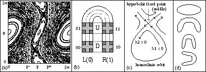
Fig 6 : (a) Chirikov map (K = .9716) displays both chaotic
and quasi-periodic orbits at a given energy. Note the elliptic fixed points
(surrounded by stable elliptic orbits), hyperbolic fixed points (forming
X's down the centre), and chaotic obits (stippled) all coexistent in a single
system. (b) Smale horseshoe map, illustrating the fractal nature of the
mixing process. (c) Homoclinic (self-inclined) hyperbolic fixed point, (d)
Folding process in the Henon map.
The Henon map ![]() [1.31]
[1.31]
carries out a very similar process to the horseshoe construction. It can be decomposed into an area-preserving bending, followed by lateral contraction and a rotation, as illustrated in fig 6(d).
(d) Quasiperiodicity, Stochasticity & Chaos
It is important to be able to distinguish chaotic systems from systems which may have both multiple periodicity and a degree of external noise or stochastic behavior. We have seen that the presence of external noise suppresses the higher-order periodic attractors, thus requiring further tests to eliminate hidden periodicities.
The power spectrum is one measure of the difference between chaos and quasi-periodic motion. The Liapunov exponent can also be used. In a purely stochastic process in which xn is subsequently distributed randomly across all possible values of xn+1, the Liapunov exponent will be . By contrast, in a quasi-periodic system with many periodic attractors, the Liapunov exponents should all be less than 1. For chaotic systems some of the Liapunov exponents should have positive finite values. These can be calculated indirectly as follows : We firstly use an xn+1, xn plot of a time-series to build up a profile of the transfer function xn+1 = G(xn). We then use this graph to make an empirical calculation of G'(x). Finally we can use [1.7] to get l (see fig 13(d)). Existence of chaos can also be established by demonstrating a period 3 orbit, fig 13(d) and applying the previously result that period 3 orbits imply chaos. Because the quasiperiodicity route to chaos requires only three interacting frequencies, non-linear systems with multiple frequencies have a high probability of entering a chaotic regime.
The attractor dimension also gives a measure as uncorrelated random variables should have correlation dimension . In practice however, because the variables are not completely uncorrelated, dimensions under about 7 provide evidence for deterministic chaos as opposed to purely stochastic behavior fig 16(a). Great care has to be taken however to distinguish chaos from quasi-periodic signals with perturbing noise.
Singular value decomposition of the matrix of vectors xn = xn, ... ,
xk+n can reveal periodicities or chaos in seemingly random time series.
The matrix 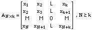
can be diagonalized ![]() U, W orthogonal :
U, W orthogonal : ![]() [1.32]
[1.32]
Where the diagonal entries in S satisfy s1 > s2, > ... > sk
> 0 and U is a rotation in k-space ( Albano et. al. 1986b) Hence applying
this rotation to the vectors xn to get ![]() should not change
the correlation dimension.
should not change
the correlation dimension.
Since the rotated vectors 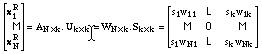 [1.33]
in the event that the singular values si have an abrupt order of magnitude decrease after sj then the rotated vectors can be reduced to their first j components. This method can sometimes unveil low-dimensional or quasi-periodic dynamics with perturbing noise as opposed to high-dimensional noise, as illustrated in fig 7 in which rotation using singular decomposition reduced the dimension from unsaturated (d2>7) to about 2.6 (Albano et. al. 1986b).
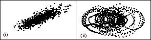
Fig 7: Singular decomposition rotation converts noisy xn+1-xn
plot (i)
into near quasi-periodic plot ![]() (ii).
(ii).
Singular value decompositions can under suitable conditions be used on
their own to estimate dimensions, but several systems such as the logistic
and Henon maps do not give easily-separated singular values (Mees et. al.
1987). An alternative strategy to improve time series estimates of correlation
dimension is to use singular-value decomposition to rotate the vectors and
choose a cut-off in the singular values at for example 10^-4 (Albano et.
al. 1988) and subsequently vary the window length in the log![]() - log
- log ![]() plot
to maximize the slope plateau.
plot
to maximize the slope plateau.
(e) Chaos at the Quantum Level and Reduction
of the Wave Packet. Quantum systems differ fundamentally from the
classical case. While the evolution of the system proceeds according to
a deterministic Hamiltonian equation : ![]() [1.34]
[1.34]
creation and destruction of quanta, particularly in the measurement process,
result in causality violations in which the probability interpretation![]() [1.35]
[1.35]
constitutes the limits on our knowledge of the system. This results in a stochastic-causal model, in which measurement collapses the wave function from a superposition of possible states into one of these states. While quantum-mechanics predicts each event only as a probability, the universe appears to have a means to resolve each reduction of the wave-packet uniquely, which I will call the principle of choice. This is the subject of Schrödinger's famous cat paradox, in which quantum mechanics predicts a cat killed as a result of a quantum fluctuation is both alive and dead with certain probabilities, while we find it is only one : alive, or dead!
Repeated attempts to model a variety of quantum analogues of classical chaotic systems have revealed significant differences which prevent the full display of chaotic dynamics. For example, the quantum kicked rotator, the analogue of the Chirikov map displays two types of solution, one rationally periodic with a parabolic gain in energy, and the other irrational with only non-diffusive almost-periodic motion. Quantum tunneling (Giesel et. al. 1986) and level repulsion (Schuster 1986) both tend to inhibit the chaotic dynamics of such systems .
The case of the Hydrogen atom in a microwave field (Casati et. al. 1986, Pool 1989) gives the closest approximation to chaos, including quantum diffusion. However numerical simulation of the quantum system remains entirely time-reversible and will regain the initial conditions, for example by phase reversal of the Fourier expansion, unlike the non-reversibility of the classical solution. Laser stimulation of molecules such as acetylene (Pique et. al. 1987) also displays borderline chaos in the fine spectra, supporting the notion that more complex molecules may display quantum chaotic phenomena under stimulation.
However it is the stochastic wave-reduction aspect of quantum mechanics which appears to underpin the uncertainty found in classical chaos. The statistical mechanics of molecular systems ultimately derives its randomness from Heisenberg uncertainty:
![]() [1.36]
[1.36]
in the form of wave-packet reduction. The position of a molecule is thus uncertain as a result of the spreading of its wave function. This uncertainty is unstably reflected in subsequent kinetic encounters causing e-small perturbations of a classically chaotic system. One of the important roles of classical chaos may thus be the amplification of quantum uncertainty into macroscopic indeterminacy. Ultimately sensitive-dependence in classical systems will result in quantum inflation, the amplification of quantum fluctuation into global perturbations of the dynamic.