 (1/2), 4] is regarded as one piece of output (a vector with two
elements, or a 1 by 2 matrix) in the following.
(1/2), 4] is regarded as one piece of output (a vector with two
elements, or a 1 by 2 matrix) in the following.
This guide is intended to quickly get you familiar with the way that MATLAB works. MATLAB has many features that we cannot cover in a short guide, but the guide should be enough to get you started. The program has a very nice on-line help facility for more detailed information.
To start MATLAB, you can double-click the icon on the desktop. If the icon is not there, you can access it by clicking on the Start button at the bottom left of the screen. Click on “All Programs”. In the menu that appears, select MATLAB, and after this, click MATLAB again.
In the MATLAB window you see a Command Window with a flashing cursor. You should work through this guide by copying the commands into the Command Window. You could retype, or just use copy and paste from the web site.
Enter the following. You could copy and paste into MATLAB, or retype.
>> 354/36
ans = 9.8333 |
MATLAB likes to do approximate calculations. You can get exact results by using the sym function:
>> sym(’354/36’)
ans = 354/36 |
and then simplify the result using simplify:
>> simplify(ans)
ans = 59/6 |
To obtain approximate results again, use the function double:
>> double(ans)
ans = 9.8333 |
The variable ans refers to the result of the last calculation. To save more results you need to assign explicitly, like this:
>> a=sym(’59/6’)
a = 59/6 |
which assigns to the variable a instead of ans. Lets take some square roots: by default approximate values are used:
>> sqrt(118/69)
ans = 1.3077 |
Using the command format long we can get more decimal digits; using format short the default is used again.
>> format long
>> sqrt(118/69) ans = 1.30772509631659 |
Since the variable a was already symbolic it will stay that way, even after taking a square root:
>> sqrt(a)
ans = 1/6*354^(1/2) |
This can’t be evaluated exactly so MATLAB just rationalises the denominator. As was shown above, you can try to further simplify expressions using MATLAB’s simplify, but here we see no improvements:
>> simplify(ans)
ans = 1/6*354^(1/2) |
MATLAB has all the mathematical functions and operations that you find on a calculator, and many more:
>> factorial(3)
ans = 6 >> sym(’exp(1)’) ans = exp(1) >> log(2.3) ans = 0.83290912293510 >> simplify(sym(’sin(pi/4)’)) ans = 1/2*2^(1/2) >> log2(16) ans = 4 >> simplify(sym(’cos(pi/3)’)) ans = 1/2 >> simplify(sym(’arctan(1)’)) ans = 1/4*pi |
Some other useful functions are floor, ceil, frac. floor(x) is the greatest integer less than or equal to x. ceil(x) is the least integer greater than or equal to x. frac(x) is the fractional part of x.
Commas between expressions yield output on different lines. brackets keep the
output on the same line. In fact, brackets are used to put things in a vector or
matrix, so [3(1/2), 4] is regarded as one piece of output (a vector with two
elements, or a 1 by 2 matrix) in the following.
>> 3, [sqrt(sym(3)) 4], 2^3
ans = 3 ans = [ 3^(1/2), 4] ans = 8 |
A semicolon suppresses the preceding output, Quite useful for doing a bunch of calculations in one step:
>> 4; 2^3
ans = 8 |
There are two ways to use MATLAB’s Help feature. To find out more about a MATLAB function just enter help followed by the function name. Try this:
>> help log
|
The other way to get help is through the help menu. This starts a help browser that lets you search for information about MATLAB.
The functions expand, simplify, normal and factor are very useful for manipulating expressions. Here we are manipulating symbolic expressions that involve the variable x. However, by default MATLAB assumes that a variable is numerical, so we need to explicitly tell MATLAB that it is symbolic. The command syms x does this. Multiple variables can be declared symbolic in the same way, using, for instance, syms x y to declare the variables x and y as symbols.
>> syms x
>> expand((2+x)^3-(5+2*x)^2+17) ans = -8*x+2*x^2+x^3 >> factor(ans) ans = x*(x+4)*(x-2) >> simplify((2*x^2+3*x+1)/(x+1)^2) ans = (2*x+1)/(x+1) >> pretty(ans) 2 x + 1 ------- x + 1 |
As you can see, pretty shows a more readable representation of the answer. The function simple rewrites an expression, here

in many different ways:
>> simple(2/x + 3*(x+1)/(x^2+1))
... >> simplify(sin(x)^2+cos(x)^2) ans = 1 |
The File menu of MATLAB allows you to save the current MATLAB state as a binary “MAT-file”, using the “Save Workspace As” menu option. The contents of all the variables are saved.
If you just want to keep a log of the commands you were giving in a text file, use the diary(’file’) command. This command produces a file, that can be opened with a text editor (such as NotePad if you use a PC), or a word processing program (such as MS Word). You could also just copy and paste everything into a word processing program. If you need to use your MATLAB statements again, just copy and paste back into MATLAB. The commands diary off and diary on toggle the recording.
A variable can be assigned a value by using the symbol =
>> syms x y
>> x=2 x = 2 >> a=x^2+y a = 4+y >> y=5 y = 5 |
If you ask MATLAB for the value of a, it won’t evaluate it with the new value of y
>> a
a = 4+y |
but you can ask it to evaluate it with the eval command.
>> eval(a)
ans = 9 |
Variables need not just have numerical values in MATLAB. They can be equated to any MATLAB expression.
>> syms z B
>> B=z^2+5*z+1 B = z^2+5*z+1 |
We could substitute the value z = 5 into this expression using MATLAB’s subs command:
>> subs(B,z,5)
ans = 51 |
You list all the symbolic variables that you are using with the command syms without any arguments. Similarly, the command who lists all variables, including the numerical ones.
>> syms
’B’ ’a’ ’x’ ’y’ ’z’ |
The variable a became symbolic automatically, because it derives from x and y. Variables can be deleted from memory and you’ll need to do this from time to time when you use variables for different things. The semicolon at the end of the command suppresses the “ans=” output.
>> clear B a z;
|
Now if we enter these variables then MATLAB complains that they do not exist.
>> B
??? Undefined function or variable ’B’. |
A function can be seen as an expression, e.g. the function f(x) = x2 + 1 can be written as y = x2 + 1. Then we have to use the subs command to evaluate the function at a particular x value.
>> syms x y
>> y=x^2+1 y = x^2+1 >> subs(y,x,2) ans = 5 >> syms a >> subs(y,x,a) ans = a^2+1 |
Composition of functions is also possible, using compose. As an example, to compute h = f ∘ g, with

just do this:
>> h=compose(y,2*x)
h = 4*x^2+1 >> subs(h,x,3) ans = 37 |
In functions of two or more variables you can substitute like this:
>> syms x y
>> g=x*y g = x*y >> subs(g,{x,y},{2,5}) ans = 10 |
Functions are easily plotted with ezplot.
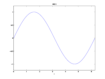
>> syms x
>> ezplot(sin(x), [-pi pi]) |
You can use the axis command to specify the y-axis:
>> ezplot((x+1)/(x^2-5), [-8 8])
>> axis([-8 8 -10 10]) |
The default title of a graph is just the mathematical expression for what is being graphed. But you can change this, and the axis labels using the commands xlabel, ylabel, and title:
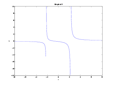
>> xlabel(’x’)
>> ylabel(’f(x)’) >> title(’Graph of f’) |
You can plot functions of two variables with ezsurf:
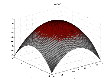
>> syms x y
>> ezsurf(1-x^2-y^2,[-2 2]) |
The function diff differentiates:
>> syms a x
>> diff(x^3) ans = 3*x^2 |
Higher order derivatives are computed like this 4th derivative
>> diff(exp(a*x),x,4)
ans = a^4*exp(a*x) >> diff(sin(x)) ans = cos(x) >> g=3*cos(x^2+1); >> diff(g,2) ans = -12*cos(x^2+1)*x^2-6*sin(x^2+1) |
Use int for indefinite or definite integrals:
>> syms x
>> int(x^2,x) ans = 1/3*x^3 |
This is the antiderivative. Don’t forget to include an arbitrary constant! To calculate

just do this:
>> int(x^2,0,1)
ans = 1/3 |
Infinity is represented by inf:
>> int(1/(1+x^2),-inf,inf)
ans = pi |
Sometimes there is no nice expression for an integral. In this case MATLAB just returns the formula that you gave it. But you could still get a numerical approximation to a definite integral.
>> int(exp(-x^3),0,3)
ans = 3/4*3^(1/2)*exp(-27/2)*WhittakerM(1/6,2/3,27)+1/27*3^(1/2)*exp(-27/2)* WhittakerM(7/6,2/3,27) >> double(ans) ans = 0.89297951156918 |
>> syms a b c x
>> z=solve(’(x^2+2*x+2)/(x+3) = 2*x+1’) z = -5/2-1/2*21^(1/2) -5/2+1/2*21^(1/2) |
There are two solutions. To pick out the first solution, try this:
>> z(1)
ans = -5/2-1/2*21^(1/2) >> solve(’tan(y) = 1’) ans = 1/4*pi |
To solve a system of equations, separate them by commas:
>> [x,y]=solve(’2*x^2+y=5’, ’x+3*y=10’)
x = -5/6 1 y = 65/18 3 >> solve(’a*x^2+b*x+c=0’,x) ans = 1/2/a*(-b+(b^2-4*a*c)^(1/2)) 1/2/a*(-b-(b^2-4*a*c)^(1/2)) |
>> limit(sin(x)/x,x,0)
ans = 1 >> limit((3*x^2+6)/(2*x^2+sin(x)), x, inf) ans = 3/2 >> limit(x/abs(x),x, 0) ans = NaN |
NaN means “Not a Number”. It implies that the limit does not exist. Left or right limits may exist even if the actual limit does not, and they are easy to compute:
>> limit(x/abs(x),x,0, ’left’)
ans = -1 |
MATLAB denotes i = sqrt(-1) with the symbol i.
>> solve(’x^2+x+1=0’)
ans = -1/2+1/2*i*3^(1/2) -1/2-1/2*i*3^(1/2) |
Real and imaginary parts of complex numbers are found with real and imag and the conjugate with conj.
>> [real(ans), imag(3+2*i), conj(4+7*i)]
ans = [ 0, 2, (4)-(7)*i] |
The absolute value of a complex number is found with abs and the argument with arg:
>> [abs(sym(1)+5*i), abs(2+i)]
ans = [ 26^(1/2), sqrt(5)] |
To compute

use MATLAB’s symsum function:
>> syms n
>> symsum(1/n^2,1,inf) ans = 1/6*pi^2 >> syms k >> simplify(symsum(k,1,n)) ans = 1/2*n^2+1/2*n >> symsum(n*exp(-n),n,1,5) ans = exp(-1)+2*exp(-2)+3*exp(-3)+4*exp(-4)+5*exp(-5) >> symsum(sin(n)/n,n,1,inf) ans = sum(sin(n)/n,n = 1 .. Inf) |
Sometimes MATLAB can’t give a nice expression for a sum...
>> symsum(1/(n^4+sqrt(n)),1,inf)
ans = sum(1/(n^4+n^(1/2)),n = 1 .. Inf) |
...but MATLAB can still give a numerical approximation:
>> vpa(ans,10)
ans = .5769509212 |
To compute 5 terms Taylor Series of cos(t) about t = π, enter
>> syms t
>> taylor(cos(t),t,pi,5) ans = -1+1/2*(t-pi)^2-1/24*(t-pi)^4 >> taylor(cos(t)/t^2, 0, 4) ??? Error using ==> sym.taylor Error, does not have a taylor expansion, try series() |
Matrices and vectors are written as in these examples:
>> syms A b c
>> A=[1 5 7; 6 1 4], b=[1;7;9], c=[6 7] A = 1 5 7 6 1 4 b = 1 7 9 c = 6 7 |
To get the entries of matrices and vectors, use
>> [A(1,3), b(3), c(2)]
ans = 7 9 7 |
MATLAB makes use of +, *, - and  for matrix algebra.
>> A*b, c*A
ans = 99 49 ans = 48 37 70 >> syms F G >> F=[sym(1) 3; 4 2], G=[sym(-2) 1; 5 2] F = 1 3 4 2 G = -2 1 5 2 >> F+G, F*G, 2*F-3*G, F^(-1), inv(F) ans = [ -1, 4] [ 9, 4] ans = [ 13, 7] [ 2, 8] ans = [ 8, 3] [ -7, -2] ans = [ -1/5, 3/10] [ 2/5, -1/10] ans = [ -1/5, 3/10] [ 2/5, -1/10] |
Notice that F (-1) and inv(F) both give the inverse of a matrix. You can also
compute the exponential of a square matrix:
(-1) and inv(F) both give the inverse of a matrix. You can also
compute the exponential of a square matrix:
>> expm(t*F)
ans = [ 4/7*exp(-2*t)+3/7*exp(5*t), 3/7*exp(5*t)-3/7*exp(-2*t)] [ 4/7*exp(5*t)-4/7*exp(-2*t), 3/7*exp(-2*t)+4/7*exp(5*t)] |
In MATLAB, you can construct a row vector with a collection of MATLAB expressions separated by commas:
>> mysequence = [sin(t), 1, sqrt(9), 4*t^3]
mysequence = [ sin(t), 1, 3, 4*t^3] |
This is a single MATLAB object. But parts of it can be extracted. To get the fourth element:
>> mysequence(4)
ans = 4*t^3 |
Sometimes vectors involve repeated elements. MATLAB’s ones function can help with that for us: To put n copies of an element into a vector, just enter the object multiplied by ones(1,n).
>> syms x y t
>> [x, y * ones(1,2), t * ones(1,3)] ans = [ x, y, y, t, t, t] |
The n:m expression, where n and m are natural numbers provides the sequence
n,n + 1,n + 2,…,m. You can also square a vector (or matrix) element-wise, by
using . :
:
>> [3:6].^2
ans = 9 16 25 36 |
Here are some more examples:
>> [1,2,log(t),5], mylist=1+0.2*(0:5)
ans = [ 1, 2, log(t), 5] mylist = Columns 1 through 5 1.00000000000000 1.20000000000000 1.40000000000000 1.60000000000000 1.80000000000000 Column 6 2.00000000000000 |
It’s easy to pick out individual components:
>> mylist(2), mylist(2:5)
ans = 1.20000000000000 ans = 1.20000000000000 1.40000000000000 1.60000000000000 1.80000000000000 |
Here are some other operations that you can now do on matrices and vectors:
>> syms u v
>> u=[1;2;3], v=[-2;4;2] u = 1 2 3 v = -2 4 2 >> dot(u,v) ans = 12 >> cross(u,v) ans = -8 -8 8 >> syms A >> A=[sym(1) 5 7 8; 6 1 4 1] A = [ 1, 5, 7, 8] [ 6, 1, 4, 1] >> A’ ans = [ 1, 6] [ 5, 1] [ 7, 4] [ 8, 1] >> syms G V D >> G=[sym(-2) 1; 5 2]; [V,D]=eig(G) V = [ 1, -1] [ 5, 1] D = [ 3, 0] [ 0, -3] |
The function eig lists each eigenvalue in D, and the corresponding eigenvectors as rows in V. In this case the eigenvalues are 3 and -3.
The characteristic polynomial of G is found using poly:
>> poly(G)
ans = x^2-9 |
We’ve already seen how to solve general equations. To solve linear equations (which can be written in the form Ax=b), use
>> b=[sym(1);2]
b = 1 2 >> A\b ans = 9/29 4/29 0 0 |
We have already seen that MATLAB has lots of built-in functions. We can also build our own functions, either using a seperate file or directly. Here we only treat the direct method, anonymous functions. Anonymous functions are declared using an @-sign.
E.g., the function f(x) = x2 + 1 can be thought of as an operation that maps a
number x to a number x2 + 1, i.e. x x2 + 1.
>> f=@(x)x^2+1
f = @(x)x^2+1 >> f(2) ans = 5 >> syms a >> f(a) ans = a^2+1 |
Composition of these functions is also possible. As before, to compute h = f ∘ g, with

you can use compose like this:
>> g=@(x)2*x
>> h = @(x)compose(f(x),g(x)) h = @(x)compose(f(x),g(x)) >> h(x) ans = 4*x^2+1 |
or directly using
>> h=@(x)f(g(x))
h = @(x)f(g(x)) >> h(3) ans = 37 |
Functions of two or more variables can be written like this:
>> g=@(x,y)x*y
g = @(x,y)x*y >> g(2,5) ans = 10 |
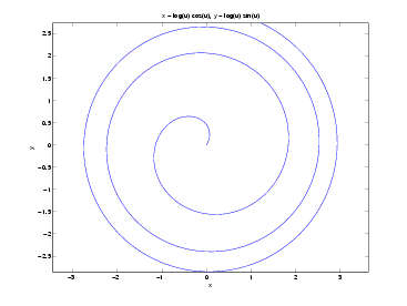
Parametrised Curves: This function defines a parametrised spiral:
>> syms R u
>> R=@(u) [log(u)*cos(u), log(u)*sin(u)] R = @(u) [log(u)*cos(u), log(u)*sin(u)] |
Use ezplot to plot such a curve.
ezplot(R(u), [1 20])
|
Differential equations are not handled with dsolve. We need to specify the differential equation and function to be found. We do this with the function dsolve:
>> logistic = ’Dy=y*(1-y)’
logistic = Dy=y*(1-y) >> dsolve(logistic) ans = 1/(1+exp(-t)*C1) |
All solutions are of this form.
You can also specify initial conditions. Note that here we have entered y(0)=1/10 instead of y(0)=0.1. You usually get better answers if you use exact arithmetic in symbolic calculations. Follow this link to see what happens if you don’t.
>> dsolve(logistic, ’y(0)=1/10’)
ans = 1/(1+9*exp(-t)) |
This Volterra-Lotka system models the interaction between predators (population size y) and prey (population size x).
It’s an example of a system of ODEs which doesn’t have a solution that can be written down in terms of common functions. But we can make use of MATLAB’s numerical routines for solving it.
First we need to write a function for the RHS of the differential equations. Think of Z as being the vector (x,y). Thus the first component of Z is Z(1) = x and the second component is Z(2) = y.
>> f=@(t,Z) [Z(1)*(2-Z(2));Z(2)*(-3+Z(1))]
f = @(t,Z) [Z(1)*(2-Z(2));Z(2)*(-3+Z(1))] |
Now to get the solution at time t = 1, we call ode45. Note that the initial condition is specified by the vector (1, 4) and the time interval for the solution is [0, 1].
>> [t,Z]=ode45(f,[0 1],[1;4]);
>> length(t) ans = 41 >> Z(41,:) ans = 1.4351 0.5034 |
This is just the solution value at time t = 1. This isn’t much use for plotting. To get a plot of the solution values over a range of time values, just use plot:
>> plot(t,Z)
|